spesim workflow: basic → intermediate → advanced • spesim

This vignette gives a structured overview of what spesim can do, arranged as a progression from basic (fast, minimal outputs) through intermediate (common teaching / exploration workflows) to advanced (full reporting and diagnostic panels).

It is meant as a map of the package: which functions are involved, what inputs and outputs to expect, and which “knobs” to turn at each stage.

Big picture workflow

Below is a compact workflow diagram showing the main pipeline.

┌──────────────────────────────┐
│ 1) Configuration             │
│   - load_config(init_file)   │
│   - or tweak list P in R     │
└───────────────┬──────────────┘
                │
                v
┌──────────────────────────────┐
│ 2) Run simulation            │
│   spesim_run()               │
│   - creates domain (or use)  │
│   - simulates individuals    │
│   - places quadrats          │
│   - builds matrices          │
└───────────────┬──────────────┘
                │
                v
┌──────────────────────────────────────────────────────┐
│ 3) Primary outputs (returned in-memory; optional disk)│
│   res$species_dist   (individual points, with species)│
│   res$quadrats       (quadrat polygons)               │
│   res$abund_matrix   (site × species table)           │
│   res$env_gradients  (gridded env fields)             │
│   res$site_coords    (quadrat centroids)              │
└───────────────┬──────────────────────────────────────┘
                │
                ├───────────── Basic: maps + matrices
                │
                ├───────────── Intermediate: derived analyses
                │                 - rank–abundance
                │                 - occupancy–abundance
                │                 - SAR
                │                 - distance–decay
                │                 - rarefaction
                │
                └───────────── Advanced: panels + report
                                  - generate_advanced_panel(res)
                                  - generate_full_report(res)

Three levels of use

Level 1 — Basic: fast, minimal, robust

Goal: run a small simulation quickly and get the essential objects back for plotting and teaching.

What you typically do

library(spesim)
#> spesim 0.5.2 loaded - try spesim_run() to generate a simulation.

# Start from a known-working example init file
init <- system.file("examples/spesim_init_basic.txt", package = "spesim")
P <- load_config(init)
#> ========== INITIALISING SPATIAL SAMPLING SIMULATION ==========

# Keep it fast (in-memory only)
P$ADVANCED_ANALYSIS <- FALSE
res <- spesim_run(P, write_outputs = FALSE, seed = P$SEED)
#> spesim: running simulation
#> Note: no non-1 interactions for species: A, B, C, D, E, F, G, H, I, J.
#> ---- Interactions Summary ----
#> Species: 10 (A..J)
#> Radius : 0
#> Non-1 entries: 0 (0.0% of 100)
#> 
#> Matrix ('.' = 1):
#>   A B C D E F G H I J
#> A . . . . . . . . . .
#> B . . . . . . . . . .
#> C . . . . . . . . . .
#> D . . . . . . . . . .
#> E . . . . . . . . . .
#> F . . . . . . . . . .
#> G . . . . . . . . . .
#> H . . . . . . . . . .
#> I . . . . . . . . . .
#> J . . . . . . . . . .
#> ------------------------------

names(res)
#> [1] "P"             "domain"        "species_dist"  "quadrats"     
#> [5] "env_gradients" "abund_matrix"  "site_env"      "site_coords"

Useful objects at this level

res$domain — sampling domain polygon
res$species_dist — individuals as sf POINTS with a species column
res$quadrats — quadrat polygons with quadrat_id
res$abund_matrix — site × species abundance table

Basic visualisations

# Domain + quadrats
plot_quadrats(res$domain, res$quadrats, title = "Quadrats")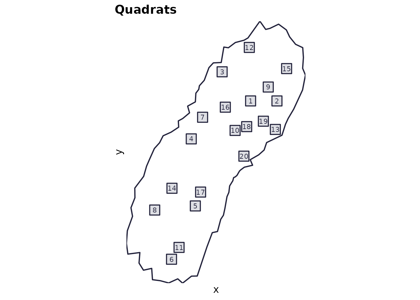

Level 2 — Intermediate: typical analyses + teaching plots

Goal: use the returned objects to compute common community-ecology summaries.

These are the same components that appear in the “advanced panel”, but here you can compute/plot them separately or integrate them into lessons.

Typical intermediate steps:

Rank–abundance (SAD):
- calculate_rank_abundance(res$species_dist, res$P)
- plot_rank_abundance(...)
Occupancy–abundance:
- calculate_occupancy_abundance(res$abund_matrix)
- plot_occupancy_abundance(...)
Species–area curve (SAR):
- calculate_species_area(res$abund_matrix)
- plot_species_area(...)
Distance–decay:
- calculate_distance_decay(res$abund_matrix, res$site_coords)
- plot_distance_decay(...)
Rarefaction:
- calculate_rarefaction(res$abund_matrix)
- plot_rarefaction(...)

Example (one intermediate product):

ra <- calculate_rank_abundance(res$species_dist, res$P)
plot_rank_abundance(ra)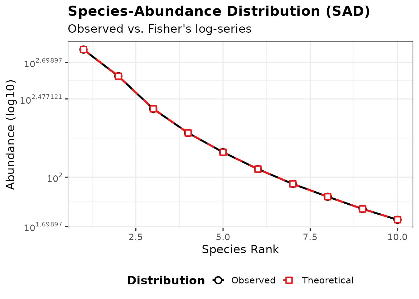

Level 3 — Advanced: full diagnostics + report

Goal: generate a compact multi-plot diagnostic panel and a human-readable report.

There are two ways to do this:

In-memory (useful for notebooks and teaching):

panel <- generate_advanced_panel(res)
print(panel)
cat(generate_full_report(res))

Write to disk (useful for “run it and inspect outputs” workflows):

# This will write timestamped outputs under out/demo_YYYYMMDD... etc.
res2 <- spesim_run(P, write_outputs = TRUE, output_prefix = "out/demo", seed = P$SEED)

What features live where?

Configuration options

“Init file” workflow: load_config("path/to/init.txt")
In-memory workflow: P <- load_config(example); P$N_SPECIES <- 10; ...

Key configuration families:

Community size + SAD: N_SPECIES, N_INDIVIDUALS, DOMINANT_FRACTION, FISHER_ALPHA, FISHER_X
Environmental filtering: GRADIENT_* plus SAMPLING_RESOLUTION, ENVIRONMENTAL_NOISE
Point processes: SPATIAL_PROCESS_A, SPATIAL_PROCESS_OTHERS and their parameters
Interactions: INTERACTION_RADIUS, INTERACTIONS_EDGELIST or INTERACTIONS_FILE
Sampling design: SAMPLING_SCHEME and scheme-specific parameters

Sampling design: quadrat placement

random: place_quadrats()
tiled: place_quadrats_tiled()
systematic: place_quadrats_systematic()
transect: place_quadrats_transect()
Voronoi-based: place_quadrats_voronoi(show_voronoi=TRUE) for teaching/visualisation

See the dedicated vignette: “Quadrat placement schemes in spesim”.

Teaching progression

A suggested progression for a lab/class:

Basic run (small, fast) → inspect res$species_dist, res$quadrats, res$abund_matrix.
Turn on gradients → show how optima/tolerance shapes spatial pattern.
Compare sampling schemes → show how design changes the observed matrix.
Turn on interactions → show how neighbourhood effects alter co-occurrence.
Run the advanced panel → interpret each diagnostic.
Read the full report → emphasise reproducibility and “what happened?” narratives.

Reproducibility notes

load_config() sets a seed (from the init file) for reproducibility.
Some intermediate analyses (e.g., SAR permutations) use randomness internally; set set.seed(...) before calling if you want exact repeatability.