Constrained ordination (db-RDA) on simulated spesim data

This vignette shows how to use spesim to generate a realistic (but known) community dataset for practising constrained ordination.

We will:

Simulate a community in an irregular domain with strong environmental gradients.
Add positive and negative interspecific interactions (local neighbourhood effects).
Compare two transect sampling designs:
- one transect aligned along the temperature gradient
- one transect set across (perpendicular to) the temperature gradient
For each design, obtain:
- a site × species abundance table
- a site × environment table (mean environment per quadrat)
Fit distance-based RDA (db-RDA) models using vegan’s capscale().
Arrange paired figures (a, b) and summarise key results in a gt table.

1) Libraries

library(spesim)
library(dplyr)
library(ggplot2)
library(vegan)
library(patchwork)

has_gt <- requireNamespace("gt", quietly = TRUE)

2) Configure a simulation with strong gradients + interactions

We start from the packaged basic init file and then modify it.

`%||%` <- function(a, b) if (!is.null(a)) a else b

init_file <- system.file("examples/spesim_init_basic.txt", package = "spesim")
P <- load_config(init_file)

# --- keep the vignette fast-ish
P$N_INDIVIDUALS <- 3000L
P$N_SPECIES <- 16L
P$N_QUADRATS <- 10L
P$SAMPLING_RESOLUTION <- 70L
P$ENVIRONMENTAL_NOISE <- 0.02
P$ADVANCED_ANALYSIS <- FALSE
quadrat_size_scale <- 0.8  # reduce quadrat side lengths by 20%

# --- strong filtering (narrow tolerances)
# A-J respond to temperature, K-L to elevation, M-P have no gradient response.
P$GRADIENT_SPECIES <- LETTERS[1:12]
P$GRADIENT_ASSIGNMENTS <- c(rep("temperature", 10), rep("elevation", 2))
P$GRADIENT_OPTIMA <- c(
  stats::setNames(seq(0.10, 0.90, length.out = 10), LETTERS[1:10]),
  K = 0.30,
  L = 0.75
)
P$GRADIENT_TOLERANCE <- 0.06

# --- local interactions
# Values < 1 weaken neighbours (negative interactions); > 1 strengthen (positive).
P$INTERACTION_RADIUS <- 1.0
P$INTERACTIONS_EDGELIST <- c(
  # negative (competition/inhibition)
  "B,A,0.80",
  "C,A,0.85",
  "D,B,0.75",
  "E,D,0.80",

  # mild background pressure for some focal species (from all neighbours)
  "B,*,0.98",
  "C,*,0.98",

  # positive (facilitation)
  "F,G,1.25",
  "G,F,1.15",
  "H,I,1.20",
  "I,H,1.10"
)

# Reproducibility
P$SEED <- 2026L

3) Two sampling designs and shared analysis helpers

To isolate the effect of sampling design, we keep the same underlying simulated community and only change transect orientation.

# Build a single deterministic domain that both designs will share.
set.seed(P$SEED)
domain <- create_sampling_domain()

# Temperature is generated from normalised coordinates:
#   temp ~ 0.7*x_norm + 0.3*y_norm
# where x_norm = (x - xmin)/(xmax-xmin), so the true gradient direction in
# x–y space depends on the domain bounding box aspect ratio.
bb <- sf::st_bbox(domain)
xrange <- as.numeric(bb["xmax"] - bb["xmin"])
yrange <- as.numeric(bb["ymax"] - bb["ymin"])

# Bearing of increasing temperature (0 = North, 90 = East)
temp_angle <- (atan2(0.7 / xrange, 0.3 / yrange) * 180 / pi) %% 360

# Perpendicular (approx. along isotherms; minimal temperature change)
across_angle <- (temp_angle + 90) %% 360

design_angles <- tibble::tibble(
  design = c("Along temperature gradient", "Across temperature gradient"),
  transect_angle_deg = c(temp_angle, across_angle)
)
design_angles

R>  [38;5;246m# A tibble: 2 × 2 [39m
R>   design                      transect_angle_deg
R>    [3m [38;5;246m<chr> [39m [23m                                     [3m [38;5;246m<dbl> [39m [23m
R>  [38;5;250m1 [39m Along temperature gradient                74.6
R>  [38;5;250m2 [39m Across temperature gradient              165.

safe_cor <- function(x, y) {
  ok <- is.finite(x) & is.finite(y)
  if (sum(ok) < 3) return(NA_real_)
  if (stats::sd(x[ok]) == 0 || stats::sd(y[ok]) == 0) return(NA_real_)
  stats::cor(x[ok], y[ok])
}

build_sampling_plot <- function(res, title, subtitle = NULL) {
  ctr <- sf::st_coordinates(sf::st_centroid(res$quadrats))
  tran <- data.frame(
    quadrat_id = res$quadrats$quadrat_id,
    x = ctr[, 1],
    y = ctr[, 2]
  ) |>
    dplyr::arrange(quadrat_id)

  ggplot() +
    geom_raster(
      data = res$env_gradients,
      aes(x = x, y = y, fill = temperature_C),
      alpha = 0.9,
      interpolate = TRUE
    ) +
    viridis::scale_fill_viridis(name = "Temperature (deg C)", option = "mako") +
    geom_sf(data = res$domain, fill = NA, colour = "grey20", linewidth = 0.4) +
    geom_path(
      data = tran,
      aes(x = x, y = y),
      linewidth = 0.45,
      colour = "white",
      alpha = 0.8
    ) +
    geom_sf(data = res$quadrats, fill = NA, colour = "black", linewidth = 0.45) +
    coord_sf(expand = FALSE) +
    theme_bw(base_size = 8) +
    labs(title = title, subtitle = subtitle, x = NULL, y = NULL)
}

build_cap_plot <- function(sc_sites, sc_bp, title) {
  p <- ggplot(sc_sites, aes(x = CAP1, y = CAP2)) +
    geom_hline(yintercept = 0, linewidth = 0.2, colour = "grey70") +
    geom_vline(xintercept = 0, linewidth = 0.2, colour = "grey70") +
    geom_point(aes(colour = temp_bin), size = 1.6, alpha = 0.85) +
    coord_equal() +
    scale_colour_brewer(palette = "RdYlBu", direction = -1, name = "Temp quartile") +
    labs(
      x = "db-RDA axis 1 (CAP1)",
      y = "db-RDA axis 2 (CAP2)",
      title = title
    )

  if (nrow(sc_bp) > 0) {
    p <- p +
      geom_segment(
        data = sc_bp,
        aes(x = 0, y = 0, xend = CAP1, yend = CAP2),
        inherit.aes = FALSE,
        arrow = arrow(length = unit(0.14, "cm")),
        linewidth = 0.3,
        colour = "black"
      ) +
      geom_text(
        data = sc_bp,
        aes(x = CAP1, y = CAP2, label = var),
        inherit.aes = FALSE,
        size = 2.5,
        vjust = -0.6
      )
  }

  p
}

analyse_design <- function(P_base, domain, label, angle_deg) {
  P2 <- P_base
  P2$SAMPLING_SCHEME <- "transect"
  P2$N_TRANSECTS <- 1L
  P2$N_QUADRATS_PER_TRANSECT <- P2$N_QUADRATS
  P2$TRANSECT_ANGLE <- angle_deg

  # Build deterministic species/environment first, then re-place
  # reduced-size transect quadrats for this comparison.
  res <- spesim_run(P2, domain = domain, write_outputs = FALSE, seed = P2$SEED, quiet = TRUE)

  quadrat_size_reduced <- as.numeric(res$P$QUADRAT_SIZE) * quadrat_size_scale
  quadrats <- place_quadrats_transect(
    domain = res$domain,
    n_transects = P2$N_TRANSECTS,
    n_quadrats_per_transect = P2$N_QUADRATS_PER_TRANSECT,
    quadrat_size = quadrat_size_reduced,
    angle = angle_deg
  )
  if (nrow(quadrats) == 0) {
    stop("Failed to place reduced-size quadrats.")
  }
  res$quadrats <- quadrats

  all_species <- LETTERS[1:P2$N_SPECIES]
  A <- create_abundance_matrix(res$species_dist, res$quadrats, all_species)
  E <- calculate_quadrat_environment(res$env_gradients, res$quadrats, sf::st_crs(res$domain))
  dat <- dplyr::left_join(E, A, by = "site")
  stopifnot(nrow(dat) == nrow(A))

  Y <- dat |> dplyr::select(-site, -temperature_C, -elevation_m, -rainfall_mm)
  X <- dat |> dplyr::select(site, temperature_C, elevation_m, rainfall_mm)
  Xz <- vegan::decostand(dplyr::select(X, -site), method = "standardize")

  cap_model <- vegan::capscale(
    Y ~ temperature_C + elevation_m + rainfall_mm,
    data = Xz,
    distance = "bray",
    add = TRUE
  )

  set.seed(P2$SEED)
  model_test <- vegan::anova.cca(cap_model, permutations = 199)
  model_p <- as.numeric(model_test$`Pr(>F)`[1])
  adj_r2 <- as.numeric(vegan::RsquareAdj(cap_model)$adj.r.squared)
  vif_vals <- tryCatch(vegan::vif.cca(cap_model), error = function(e) NA_real_)
  vif_vals <- as.numeric(vif_vals)
  vif_vals <- vif_vals[is.finite(vif_vals)]
  vif_max <- if (length(vif_vals)) max(vif_vals) else NA_real_

  sc_sites <- as.data.frame(vegan::scores(cap_model, display = "sites", scaling = 2))
  sc_bp <- as.data.frame(vegan::scores(cap_model, display = "bp", scaling = 2))
  sc_sites$site <- dat$site
  sc_sites <- dplyr::left_join(sc_sites, X, by = "site")
  sc_sites$temp_bin <- factor(dplyr::ntile(sc_sites$temperature_C, 4), labels = paste0("Q", 1:4))

  arrow_mul <- 1.3
  sc_bp$var <- rownames(sc_bp)
  if (nrow(sc_bp) > 0) {
    sc_bp$CAP1 <- sc_bp$CAP1 * arrow_mul
    sc_bp$CAP2 <- sc_bp$CAP2 * arrow_mul
  }

  cor_tbl <- sc_sites |>
    dplyr::summarise(
      cor_cap1_temp = safe_cor(CAP1, temperature_C),
      cor_cap1_elev = safe_cor(CAP1, elevation_m),
      cor_cap1_rain = safe_cor(CAP1, rainfall_mm)
    ) |>
    dplyr::mutate(design = label, .before = 1)

  metrics <- cor_tbl |>
    dplyr::mutate(
      transect_angle_deg = angle_deg,
      n_quadrats = nrow(res$quadrats),
      temp_range_C = diff(range(sc_sites$temperature_C, na.rm = TRUE)),
      adj_r2 = adj_r2,
      model_p = model_p,
      max_vif = vif_max,
      .before = cor_cap1_temp
    ) |>
    dplyr::select(
      design,
      transect_angle_deg,
      n_quadrats,
      temp_range_C,
      adj_r2,
      model_p,
      cor_cap1_temp,
      cor_cap1_elev,
      cor_cap1_rain,
      max_vif
    )

  sampling_plot <- build_sampling_plot(
    res,
    title = label,
    subtitle = sprintf("angle = %.1f deg", angle_deg)
  )
  cap_plot <- build_cap_plot(sc_sites, sc_bp, title = label)

  list(
    label = label,
    angle = angle_deg,
    res = res,
    A = A,
    E = E,
    dat = dat,
    cap = cap_model,
    cor_tbl = cor_tbl,
    metrics = metrics,
    sampling_plot = sampling_plot,
    cap_plot = cap_plot
  )
}

4) Run both designs

# 'domain' was created above so that both designs share the same geometry.
along <- analyse_design(
  P_base = P,
  domain = domain,
  label = "Along temperature gradient",
  angle_deg = temp_angle
)

R> ---- Interactions Summary ----
R> Species: 16 (A..P)
R> Radius : 1
R> Non-1 entries: 36 (14.1% of 256)
R> Asymmetry (mean |M - t(M)|): 0.009
R> 
R> Non-1 entries (sorted by |value-1|):
R>  focal neighbor value
R>      D        B  0.75
R>      F        G  1.25
R>      E        D  0.80
R>      H        I  1.20
R>      G        F  1.15
R>      I        H  1.10
R>      B        A  0.98
R>      B        C  0.98
R>      B        D  0.98
R>      B        E  0.98
R>      B        F  0.98
R>      B        G  0.98
R>      B        H  0.98
R>      B        I  0.98
R>      B        J  0.98
R>      B        K  0.98
R>      B        L  0.98
R>      B        M  0.98
R>      B        N  0.98
R>      B        O  0.98
R> ------------------------------

across <- analyse_design(
  P_base = P,
  domain = domain,
  label = "Across temperature gradient",
  angle_deg = across_angle
)

R> ---- Interactions Summary ----
R> Species: 16 (A..P)
R> Radius : 1
R> Non-1 entries: 36 (14.1% of 256)
R> Asymmetry (mean |M - t(M)|): 0.009
R> 
R> Non-1 entries (sorted by |value-1|):
R>  focal neighbor value
R>      D        B  0.75
R>      F        G  1.25
R>      E        D  0.80
R>      H        I  1.20
R>      G        F  1.15
R>      I        H  1.10
R>      B        A  0.98
R>      B        C  0.98
R>      B        D  0.98
R>      B        E  0.98
R>      B        F  0.98
R>      B        G  0.98
R>      B        H  0.98
R>      B        I  0.98
R>      B        J  0.98
R>      B        K  0.98
R>      B        L  0.98
R>      B        M  0.98
R>      B        N  0.98
R>      B        O  0.98
R> ------------------------------

Quick check that only sampling differs (same simulated species cloud):

isTRUE(all.equal(
  sf::st_coordinates(along$res$species_dist),
  sf::st_coordinates(across$res$species_dist)
))

R> [1] TRUE

5) Figure 1: sampling designs (`a`, `b`)

fig_sampling <- patchwork::wrap_plots(
  along$sampling_plot,
  across$sampling_plot,
  ncol = 2,
  guides = "collect"
) +
  patchwork::plot_annotation(tag_levels = "a")

fig_sampling

Figure 1. Quadrat placement over the temperature surface: (a) along-gradient transect, (b) across-gradient transect.

6) Full db-RDA workflow for each design

6.1 Site × species and site × environment tables

dplyr::bind_rows(
  tibble::tibble(design = along$label, n_sites = nrow(along$A), n_species_cols = ncol(along$A) - 1L),
  tibble::tibble(design = across$label, n_sites = nrow(across$A), n_species_cols = ncol(across$A) - 1L)
)

R>  [38;5;246m# A tibble: 2 × 3 [39m
R>   design                      n_sites n_species_cols
R>    [3m [38;5;246m<chr> [39m [23m                          [3m [38;5;246m<int> [39m [23m           [3m [38;5;246m<int> [39m [23m
R>  [38;5;250m1 [39m Along temperature gradient       10             16
R>  [38;5;250m2 [39m Across temperature gradient      10             16

6.2 db-RDA model summaries

along$cap

R> 
R> Call: vegan::capscale(formula = Y ~ temperature_C + elevation_m +
R> rainfall_mm, data = Xz, distance = "bray", add = TRUE)
R> 
R>               Inertia Proportion Rank
R> Total           2.330      1.000     
R> Constrained     1.426      0.612    3
R> Unconstrained   0.904      0.388    6
R> 
R> Inertia is Lingoes adjusted squared Bray distance
R> 
R> -- NOTE:
R> Species scores projected from 'Y'
R> 
R> Eigenvalues for constrained axes:
R>   CAP1   CAP2   CAP3 
R> 0.8803 0.4368 0.1086 
R> 
R> Eigenvalues for unconstrained axes:
R>    MDS1    MDS2    MDS3    MDS4    MDS5    MDS6 
R> 0.30559 0.24002 0.16262 0.11593 0.06238 0.01747 
R> 
R> Constant added to distances: 0.02267772

across$cap

R> 
R> Call: vegan::capscale(formula = Y ~ temperature_C + elevation_m +
R> rainfall_mm, data = Xz, distance = "bray", add = TRUE)
R> 
R>               Inertia Proportion Rank
R> Total          1.2468     1.0000     
R> Constrained    0.4200     0.3369    3
R> Unconstrained  0.8268     0.6631    6
R> 
R> Inertia is Lingoes adjusted squared Bray distance
R> 
R> -- NOTE:
R> Species scores projected from 'Y'
R> 
R> Eigenvalues for constrained axes:
R>    CAP1    CAP2    CAP3 
R> 0.20270 0.16131 0.05597 
R> 
R> Eigenvalues for unconstrained axes:
R>   MDS1   MDS2   MDS3   MDS4   MDS5   MDS6 
R> 0.3397 0.2131 0.1201 0.1088 0.0355 0.0096 
R> 
R> Constant added to distances: 0.02891905

7) Figure 2: db-RDA ordinations (`a`, `b`)

fig_ordination <- patchwork::wrap_plots(
  along$cap_plot,
  across$cap_plot,
  ncol = 2,
  guides = "collect"
) +
  patchwork::plot_annotation(tag_levels = "a")

fig_ordination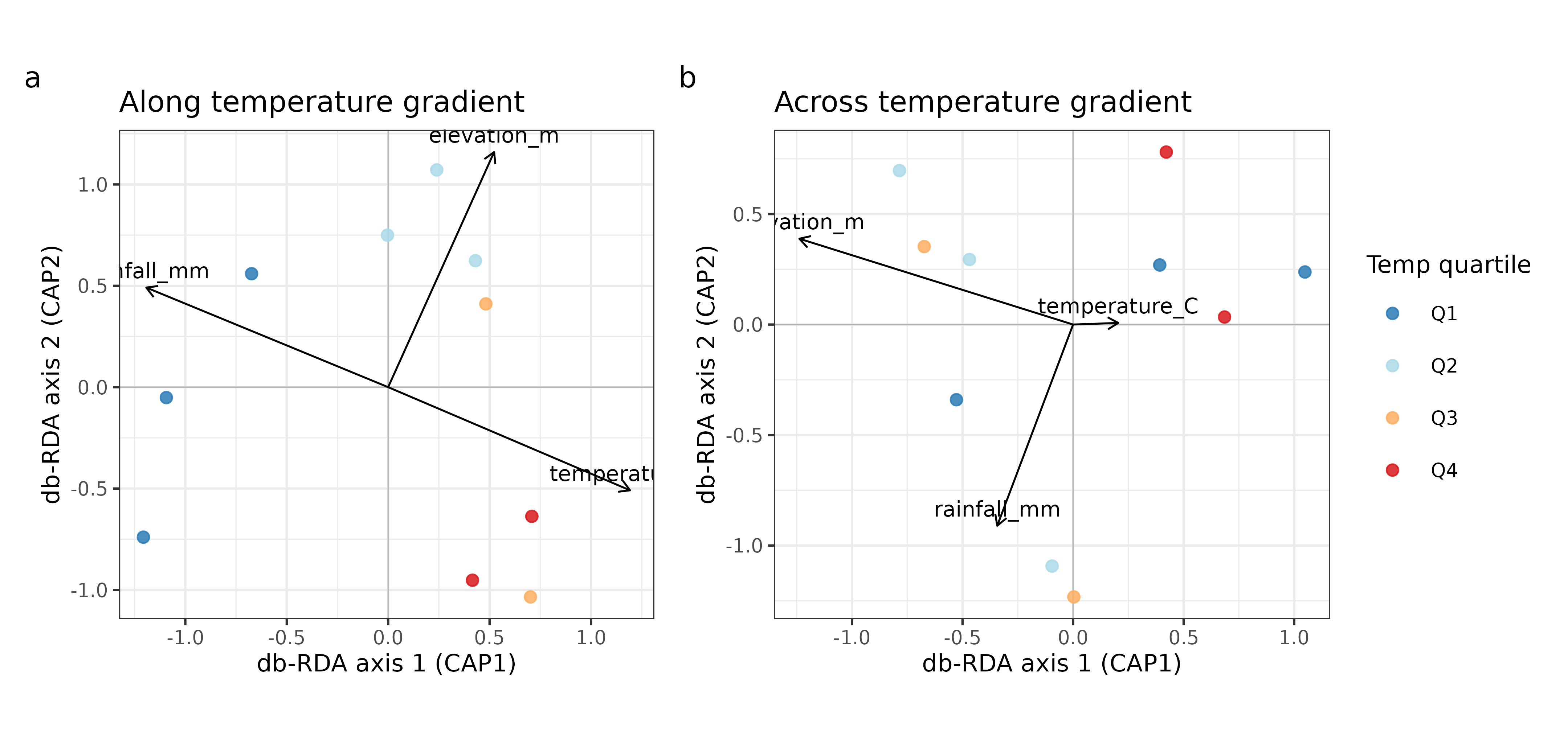

Figure 2. db-RDA ordination biplots for each sampling design.

8) Figure 3: sanity check (CAP1 vs temperature; `a`, `b`)

p_sanity_along <- ggplot(along$dat, aes(x = temperature_C, y = vegan::scores(along$cap, display = "sites", scaling = 2)[, "CAP1"])) +
  geom_point(size = 1.2, alpha = 0.85) +
  geom_smooth(method = "lm", se = FALSE, linewidth = 0.5, colour = "black") +
  theme_bw(base_size = 8) +
  labs(x = "Temperature (deg C)", y = "CAP1", title = along$label)

p_sanity_across <- ggplot(across$dat, aes(x = temperature_C, y = vegan::scores(across$cap, display = "sites", scaling = 2)[, "CAP1"])) +
  geom_point(size = 1.2, alpha = 0.85) +
  geom_smooth(method = "lm", se = FALSE, linewidth = 0.5, colour = "black") +
  theme_bw(base_size = 8) +
  labs(x = "Temperature (deg C)", y = "CAP1", title = across$label)

patchwork::wrap_plots(p_sanity_along, p_sanity_across, ncol = 2) +
  patchwork::plot_annotation(tag_levels = "a")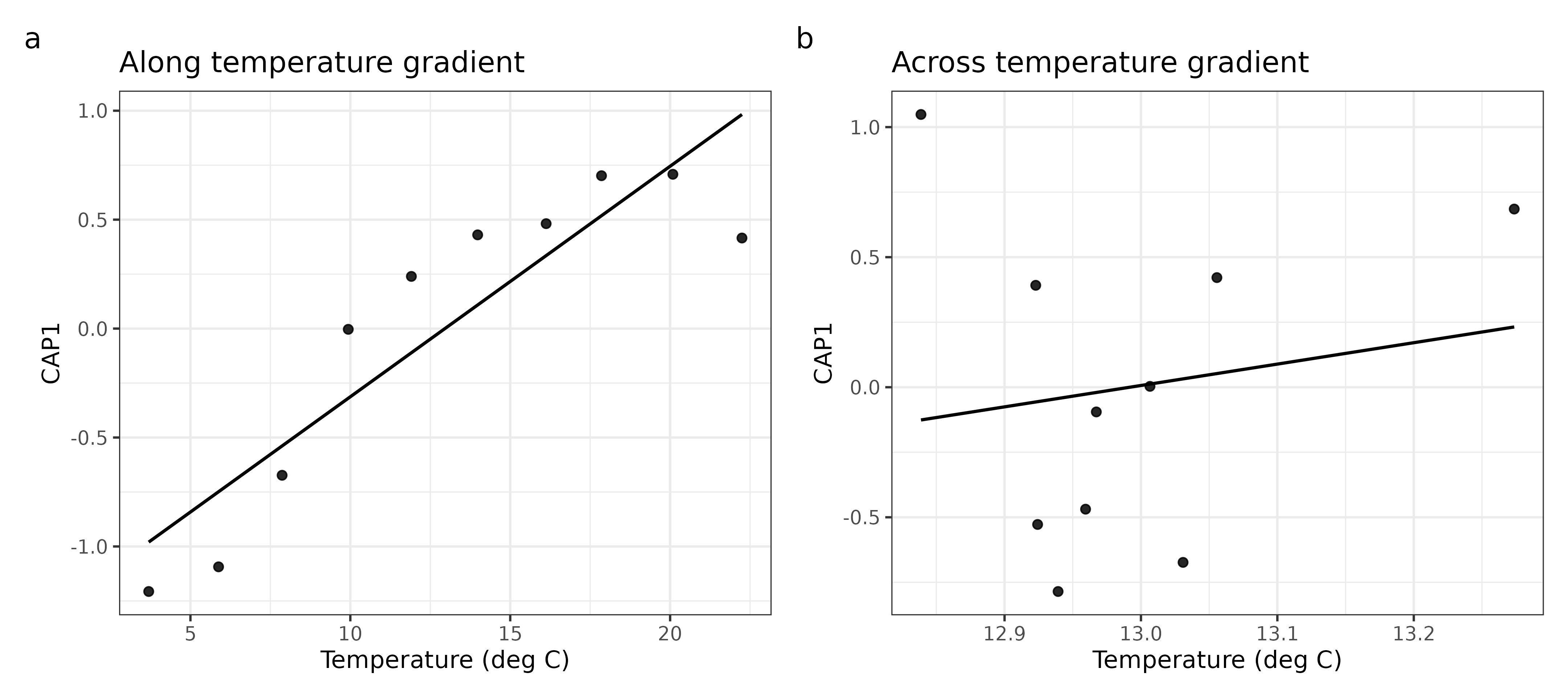

Figure 3. CAP1 tracks the sampled temperature range differently under the two designs.

9) Key results summary table (`gt`)

summary_tbl <- dplyr::bind_rows(along$metrics, across$metrics)

if (has_gt) {
  summary_tbl |>
    gt::gt() |>
    gt::fmt_number(
      columns = c(transect_angle_deg, temp_range_C, adj_r2, cor_cap1_temp, cor_cap1_elev, cor_cap1_rain, max_vif),
      decimals = 3
    ) |>
    gt::fmt_number(columns = model_p, decimals = 4) |>
    gt::cols_label(
      design = "Sampling design",
      transect_angle_deg = "Transect angle (deg)",
      n_quadrats = "Quadrats",
      temp_range_C = "Sampled temp range (deg C)",
      adj_r2 = "Adj. R^2",
      model_p = "Model p-value",
      cor_cap1_temp = "cor(CAP1, temp)",
      cor_cap1_elev = "cor(CAP1, elev)",
      cor_cap1_rain = "cor(CAP1, rain)",
      max_vif = "Max VIF"
    ) |>
    gt::tab_header(
      title = "db-RDA comparison by sampling design",
      subtitle = "Along-gradient vs across-gradient transects"
    )
} else {
  knitr::kable(summary_tbl, digits = 3)
}

Sampling design	Transect angle (deg)	Quadrats	Sampled temp range (deg C)	Adj. R^2	Model p-value	cor(CAP1, temp)	cor(CAP1, elev)	cor(CAP1, rain)	Max VIF
db-RDA comparison by sampling design
Along-gradient vs across-gradient transects
Along temperature gradient	74.603	10	18.551	0.418	0.0050	0.901	0.395	−0.901	342.292
Across temperature gradient	164.603	10	0.435	0.005	0.4450	0.154	−0.935	−0.259	1.710

10) Why this is useful for teaching

Because spesim generates: - the site × species matrix (abund_matrix), and - the corresponding site × environment matrix (via calculate_quadrat_environment()),

you can repeatedly create controlled datasets where you know the truth (strong gradients and interactions were imposed) and then practise ordination workflows that aim to recover the dominant drivers under alternative sampling designs.

Suggested exercises

Increase/decrease GRADIENT_TOLERANCE and see how the constrained R² changes.
Turn interactions off (INTERACTION_RADIUS <- 0) and compare db-RDA fits.
Compare single-transect, multi-transect, and non-transect designs to test sensitivity of constrained ordination outcomes to sampling geometry.