spesim: constrained landscapes (network/coastline MVP) • spesim

This vignette documents the new constrained-landscape features:

DOMAIN_TYPE = "network"
DOMAIN_TYPE = "coastline"
along-path distance-decay (metric = "along_path")
directional dispersal in linearized domains (DISPERSAL_DIRECTION_BIAS)
external environmental covariates (ENV_COVARIATES_FILE)

Scope and limitation

This is a linearized constrained-landscape MVP, not yet a full graph-theoretic river-network engine (no explicit edge/node topology or true network shortest-path over branches yet).

In practice, network and coastline currently use a constrained 1D coordinate embedded in a 2D polygon domain.

Base setup

library(spesim)
library(ggplot2)

pkg_file <- function(subpath, folder = c("extdata", "examples")) {
  folder <- match.arg(folder)
  p_installed <- system.file(folder, subpath, package = "spesim")
  if (nzchar(p_installed) && file.exists(p_installed)) return(p_installed)
  candidates <- c(
    file.path("inst", folder, subpath),
    file.path("..", "inst", folder, subpath)
  )
  for (p in candidates) if (file.exists(p)) return(p)
  stop("Could not find file: ", subpath, " in ", folder)
}

P0 <- load_config(pkg_file("spesim_init_basic.txt", "examples"))
P0$N_SPECIES <- 12
P0$N_INDIVIDUALS <- 400
P0$SAMPLING_SCHEME <- "tiled"
P0$N_QUADRATS <- 15
P0$QUADRAT_SIZE_OPTION <- "medium"
P0$INTERACTION_RADIUS <- 0
P0$INTERACTIONS_FILE <- NULL
P0$INTERACTIONS_EDGELIST <- NULL
P0$MODEL_FAMILY <- "neutral_hubbell_like"
P0$NEUTRAL_M <- 0.10
P0$NEUTRAL_NU <- 0.01
P0$DISPERSAL_KERNEL <- "gaussian"
P0$DISPERSAL_SCALE <- 0.45
P0$SAD_MODEL <- "zsm"
P0$ZSM_THETA <- 12

run_case <- function(P, title) {
  res <- spesim_run(P, write_outputs = FALSE, seed = P$SEED, interactions_print = FALSE)
  p_map <- plot_spatial_sampling(
    res$domain,
    res$species_dist,
    res$quadrats,
    res$P,
    show_gradient = TRUE,
    env_gradients = res$env_gradients,
    gradient_type = "temperature_C"
  ) + ggtitle(title)
  list(res = res, map = p_map)
}

Scenario A: polygon baseline

P_poly <- P0
P_poly$DOMAIN_TYPE <- "polygon"
P_poly$DISTANCE_METRIC <- "auto"

case_poly <- run_case(P_poly, "Polygon baseline (2D)")
case_poly$map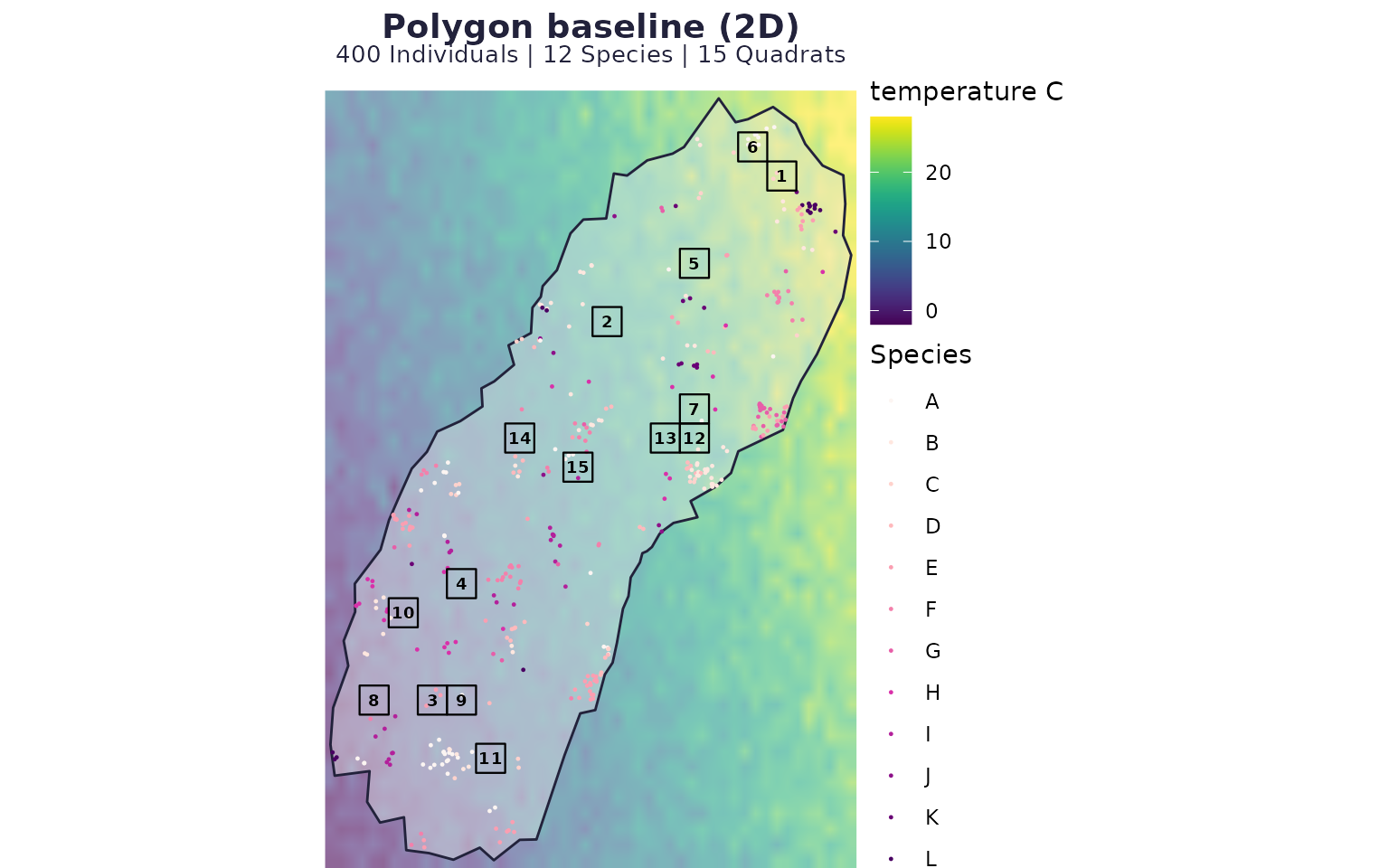

Scenario B: network-style constrained landscape (real Doubs covariates)

P_net <- P0
P_net$DOMAIN_TYPE <- "network"
P_net$LINEAR_AXIS <- "x"
P_net$LINEAR_WRAP <- FALSE
P_net$LINEAR_JITTER_SD <- 0.08
P_net$DISTANCE_METRIC <- "along_path"
P_net$ENV_COVARIATES_FILE <- pkg_file("DoubsCovariates.csv", "extdata")
P_net$ENV_DRIVERS <- c("alt", "flo", "pH", "nit", "oxy")

case_net <- run_case(P_net, "Network-like constrained landscape (Doubs data, linearized)")
case_net$map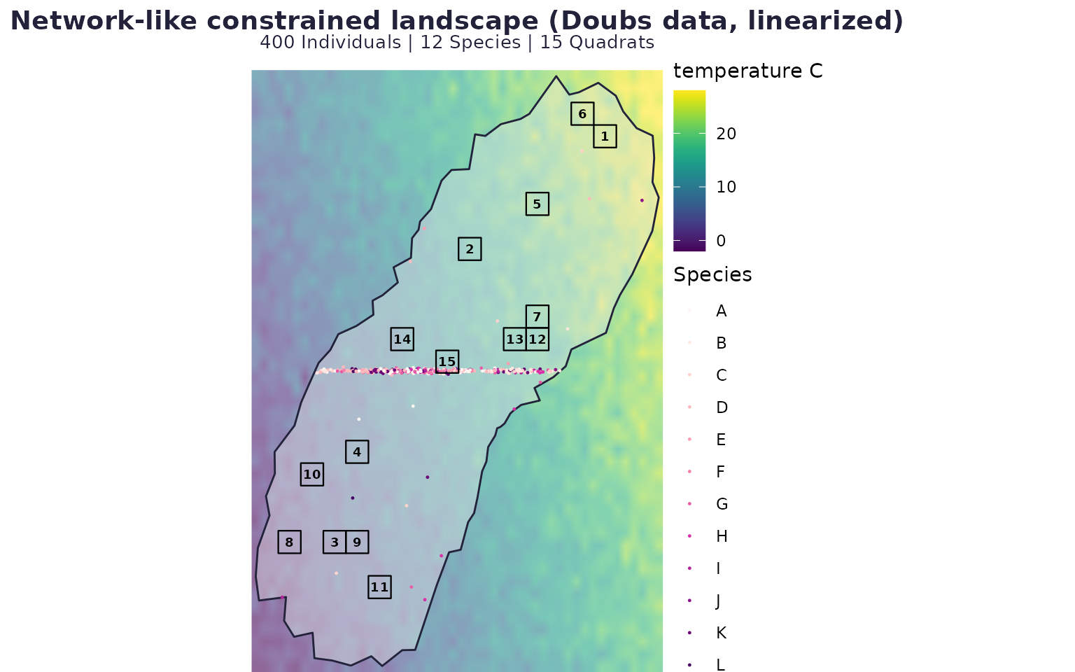

Scenario C: coastline-style constrained landscape with directional dispersal (real seaweed covariates)

P_coast <- P0
P_coast$DOMAIN_TYPE <- "coastline"
P_coast$LINEAR_AXIS <- "x"
P_coast$LINEAR_WRAP <- TRUE
P_coast$LINEAR_JITTER_SD <- 0.06
P_coast$DISTANCE_METRIC <- "along_path"
P_coast$DISPERSAL_DIRECTION_BIAS <- 0.55
P_coast$ENV_COVARIATES_FILE <- pkg_file("SeaweedCovariates.csv", "extdata")
P_coast$ENV_DRIVERS <- c("summerMean", "winterMin", "augChl")

case_coast <- run_case(P_coast, "Coastline-like constrained landscape (seaweed data)")
case_coast$map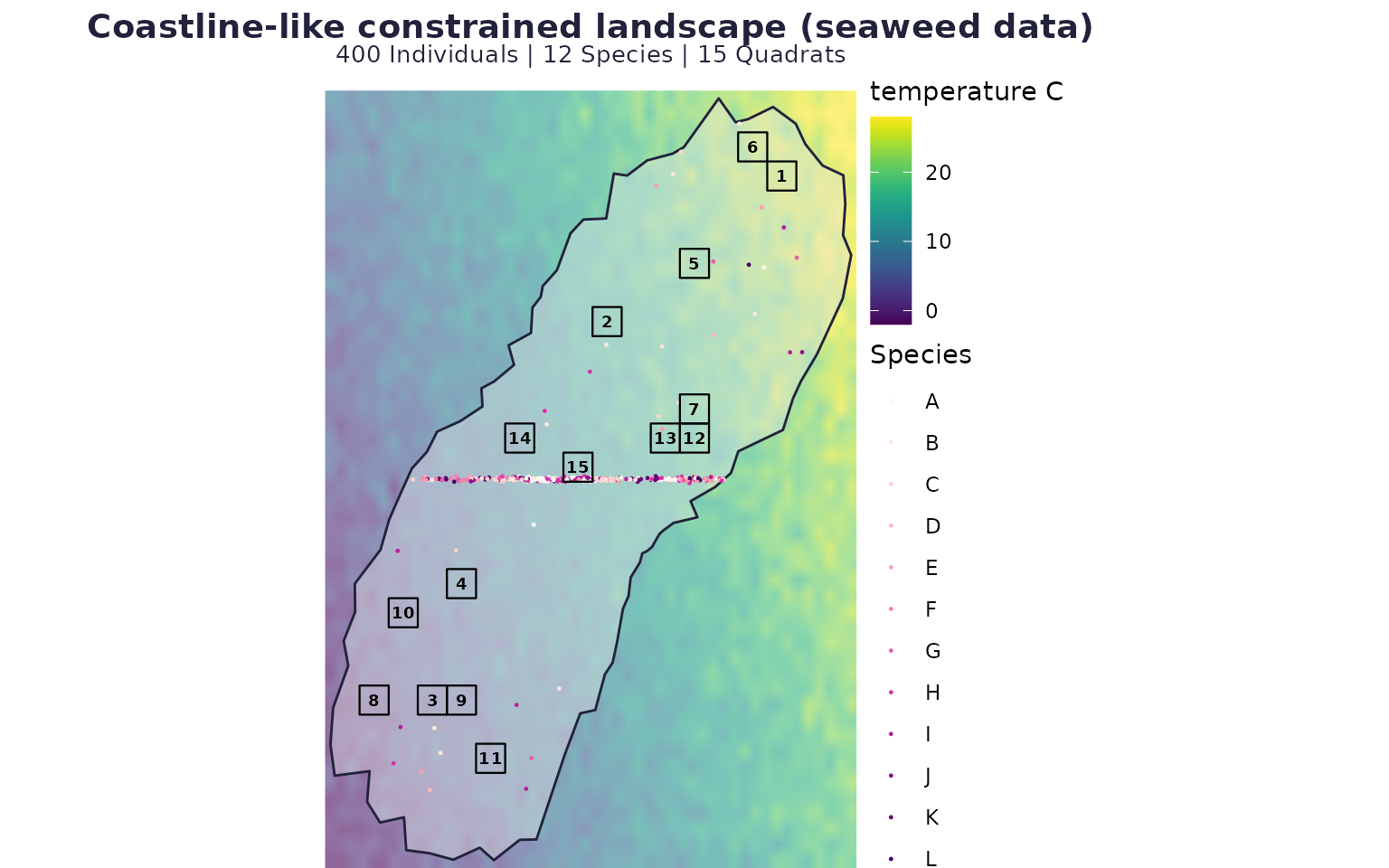

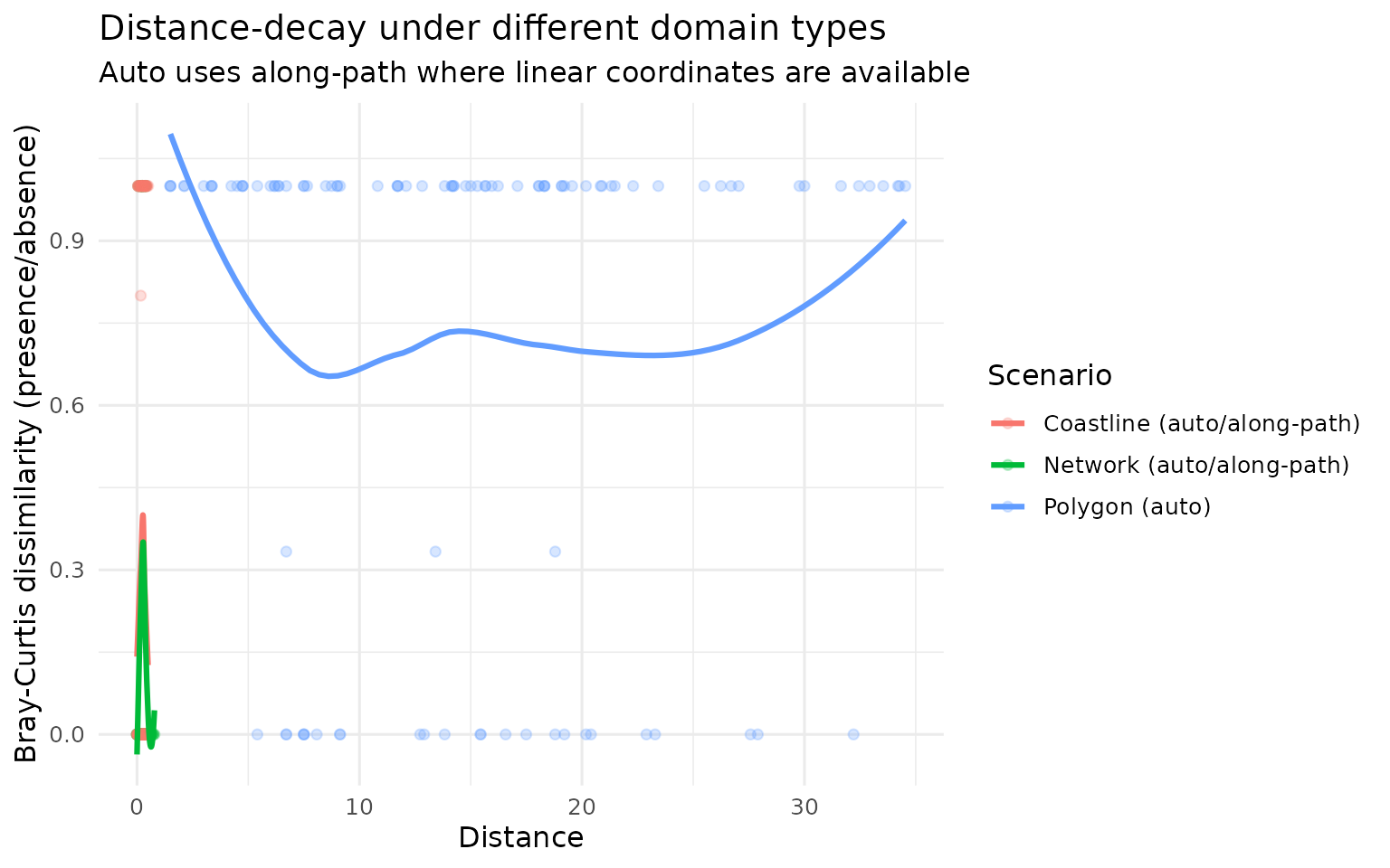
Distance-decay comparisons

Auto metric (context aware)

dd_poly_auto  <- calculate_distance_decay(case_poly$res$abund_matrix,  case_poly$res$site_coords)
dd_net_auto   <- calculate_distance_decay(case_net$res$abund_matrix,   case_net$res$site_coords)
dd_coast_auto <- calculate_distance_decay(case_coast$res$abund_matrix, case_coast$res$site_coords)

dd_auto <- rbind(
  transform(dd_poly_auto, Scenario = "Polygon (auto)"),
  transform(dd_net_auto, Scenario = "Network (auto/along-path)"),
  transform(dd_coast_auto, Scenario = "Coastline (auto/along-path)")
)

ggplot(dd_auto, aes(Distance, Dissimilarity, colour = Scenario)) +
  geom_point(alpha = 0.25) +
  geom_smooth(se = FALSE, method = "loess", span = 0.75, linewidth = 1.1) +
  theme_minimal(base_size = 12) +
  labs(
    title = "Distance-decay under different domain types",
    subtitle = "Auto uses along-path where linear coordinates are available",
    x = "Distance",
    y = "Bray-Curtis dissimilarity (presence/absence)"
  )

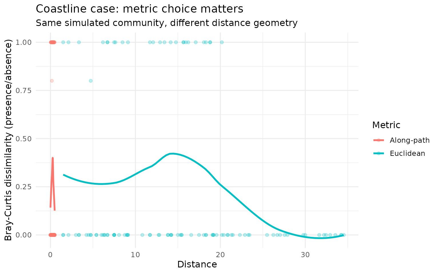
Coastline: Euclidean vs along-path on the same run

dd_coast_eu <- calculate_distance_decay(case_coast$res$abund_matrix, case_coast$res$site_coords, metric = "euclidean")
dd_coast_ap <- calculate_distance_decay(case_coast$res$abund_matrix, case_coast$res$site_coords, metric = "along_path")

dd_cmp <- rbind(
  transform(dd_coast_eu, Metric = "Euclidean"),
  transform(dd_coast_ap, Metric = "Along-path")
)

ggplot(dd_cmp, aes(Distance, Dissimilarity, colour = Metric)) +
  geom_point(alpha = 0.25) +
  geom_smooth(se = FALSE, method = "loess", span = 0.75, linewidth = 1.1) +
  theme_minimal(base_size = 12) +
  labs(
    title = "Coastline case: metric choice matters",
    subtitle = "Same simulated community, different distance geometry",
    x = "Distance",
    y = "Bray-Curtis dissimilarity (presence/absence)"
  )

Discussion

What this MVP gives now:

Constrained placement in linearized landscapes (network / coastline).
Optional wrapped distance for coastlines (LINEAR_WRAP).
Directional bias in recruitment for neutral/hybrid runs (DISPERSAL_DIRECTION_BIAS).
External node/section covariates via ENV_COVARIATES_FILE.

What is intentionally not in this MVP yet:

explicit river/coast graph topology with branched shortest paths,
edge/node attributes driving movement over true network structure,
mechanistic flow routing over network branches.

Use this MVP to test method behavior under constrained continuous gradients, then move to full graph-theoretic implementations if the ecological question requires branch-level realism.