spesim recipes: point processes (and the neutral-theory SAD helper) • spesim

This recipe shows how to:

switch the spatial point-process model for the dominant species (A) and for the remaining species,
use the neutral-theory SAD helper (SAD_MODEL = "zsm"),
use the high-level model family layer (MODEL_FAMILY) for neutral and hybrid recruitment.

The key idea is that these are orthogonal knobs:

SAD_MODEL controls how many individuals each species gets (the rank–abundance curve),
SPATIAL_PROCESS_* controls where individuals are placed in space.

Base configuration

library(spesim)
library(ggplot2)

P0 <- load_config(system.file("examples/spesim_init_complete.txt", package = "spesim"))

# Keep the vignette fast but still visually clear.
P0$N_SPECIES <- 12
P0$N_INDIVIDUALS <- 500

# Make distance–decay curves more interpretable by using a regular quadrat layout.
P0$SAMPLING_SCHEME <- "tiled"
P0$N_QUADRATS <- 16
P0$QUADRAT_SIZE_OPTION <- "medium"

# Turn off environmental filtering to keep this vignette focused on
# point-process and SAD effects (not gradient-driven turnover).
P0$GRADIENT_SPECIES <- character(0)
P0$GRADIENT_ASSIGNMENTS <- character(0)
P0$GRADIENT_OPTIMA <- NULL
P0$GRADIENT_TOLERANCE <- NULL

# Keep interactions off for clarity
P0$INTERACTION_RADIUS <- 0
P0$INTERACTIONS_FILE <- NULL
P0$INTERACTIONS_EDGELIST <- NULL

# A tiny helper to run a case and build its advanced panel.
run_case <- function(P, title) {
  res <- spesim_run(P, write_outputs = FALSE, seed = P$SEED, interactions_print = FALSE)
  panel <- generate_advanced_panel(res) + patchwork::plot_annotation(title = title)
  list(res = res, panel = panel)
}

rank_df <- function(res, label) {
  ra <- calculate_rank_abundance(res$species_dist, res$P)
  ra <- subset(ra, Source == "Observed")
  ra$Scenario <- label
  ra
}

decay_df <- function(res, label) {
  dd <- calculate_distance_decay(res$abund_matrix, res$site_coords)
  dd$Scenario <- label
  dd
}

Neutral theory in spesim (current implementation)

spesim supports two neutral-style routes:

SAD_MODEL = "zsm": theta-only neutral-like SAD helper.
MODEL_FAMILY = "neutral_hubbell_like": sequential recruitment with immigration/speciation and dispersal kernel.
MODEL_FAMILY = "hybrid": same recruitment core plus environmental sorting.

What it can do

SAD_MODEL = "zsm" gives neutral-like rank–abundance control via ZSM_THETA.
MODEL_FAMILY = "neutral_hubbell_like" gives distance–decay that emerges from dispersal-limited recruitment.
MODEL_FAMILY = "hybrid" blends dispersal limitation with environmental sorting.

What it cannot do (yet)

It is still a synthetic simulator (not calibrated population dynamics through time).
Species labels remain fixed (A..) rather than open-ended speciation lineages.
Recruitment is intentionally lightweight for method testing speed.

The practical takeaway: use SAD_MODEL = "zsm" when you only want neutral-like abundance structure; use MODEL_FAMILY = "neutral_hubbell_like" or "hybrid" when you want spatial patterns to emerge from recruitment.

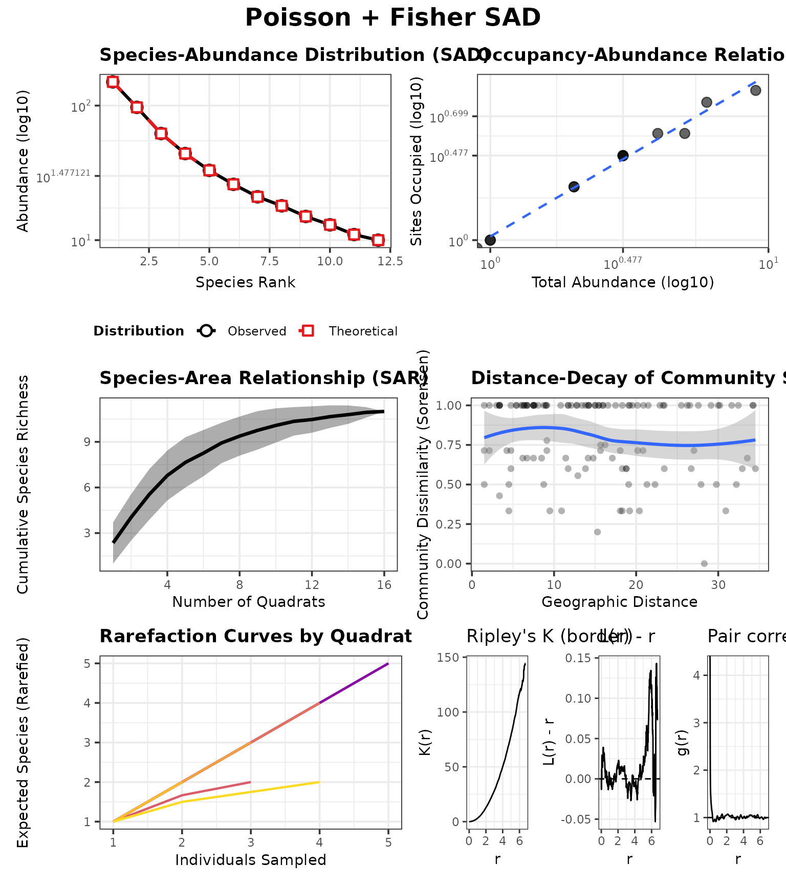
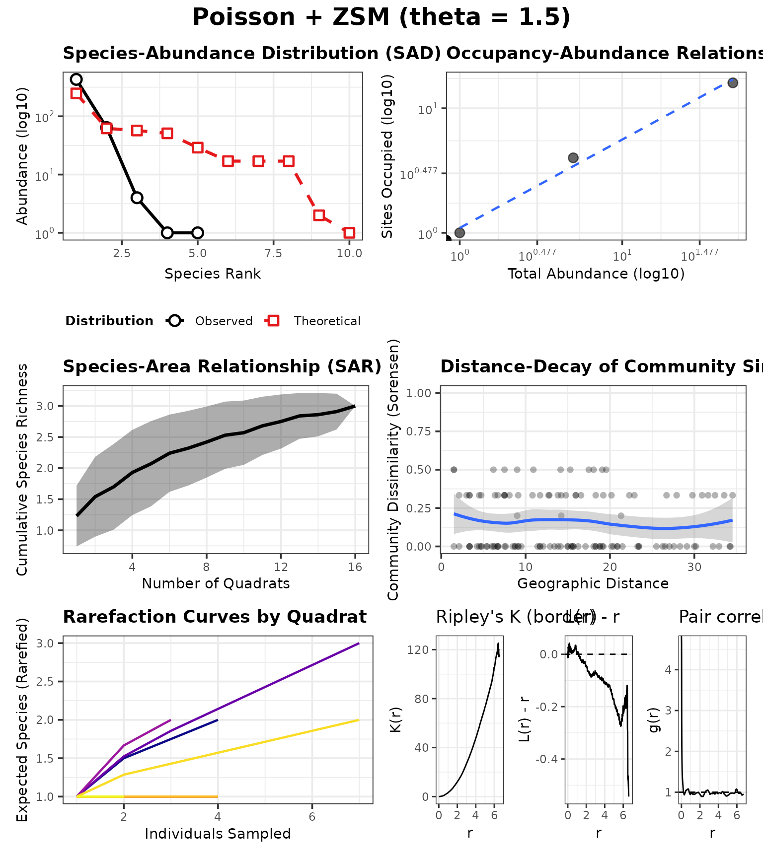
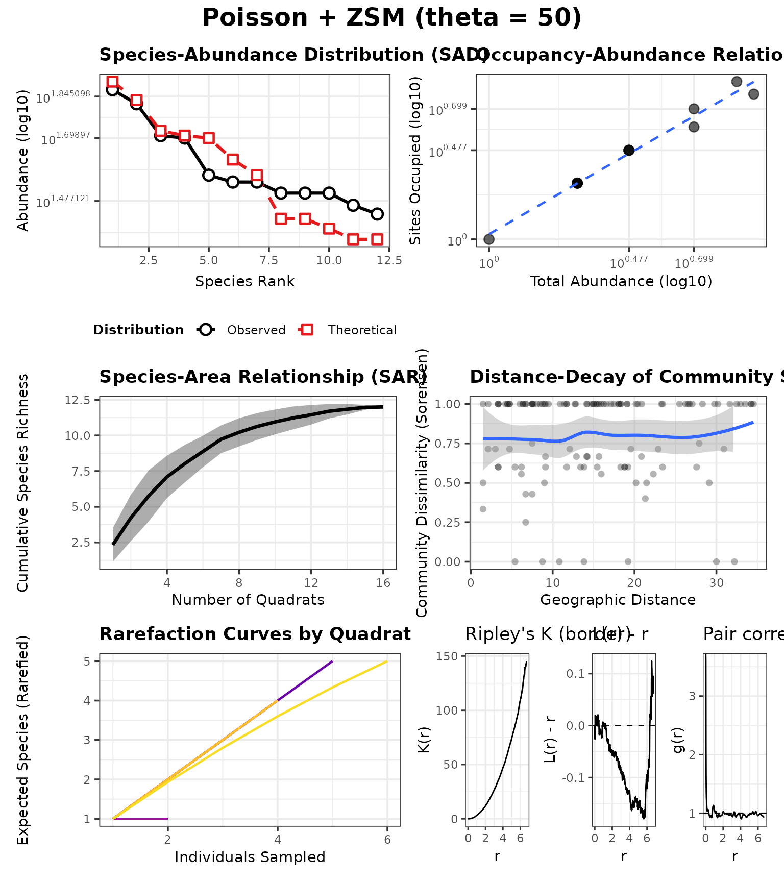
Example A: SAD differences (Fisher vs neutral-theory ZSM)

Here we hold the spatial process fixed at Poisson (CSR) so differences in the SAD plots are driven by SAD_MODEL.

P_sad <- P0
P_sad$SPATIAL_PROCESS_A <- "poisson"
P_sad$SPATIAL_PROCESS_OTHERS <- "poisson"

# Fisher baseline
P_fisher <- P_sad
P_fisher$SAD_MODEL <- "fisher"
P_fisher$DOMINANT_FRACTION <- 0.30

# Neutral-like SADs via zsm
P_zlow <- P_sad
P_zlow$SAD_MODEL <- "zsm"
P_zlow$ZSM_THETA <- 1.5
P_zlow$ZSM_M <- NA_real_

P_zhigh <- P_zlow
P_zhigh$ZSM_THETA <- 50

case_fisher <- run_case(P_fisher, "Poisson + Fisher SAD")
case_zlow   <- run_case(P_zlow,   "Poisson + ZSM (theta = 1.5)")
case_zhigh  <- run_case(P_zhigh,  "Poisson + ZSM (theta = 50)")

Rank–abundance (overlay)

ra_all <- rbind(
  rank_df(case_fisher$res, "Fisher"),
  rank_df(case_zlow$res,   "ZSM θ=1.5"),
  rank_df(case_zhigh$res,  "ZSM θ=50")
)

ggplot(ra_all, aes(Rank, Abundance, colour = Scenario)) +
  geom_line(linewidth = 1) +
  geom_point(size = 2) +
  scale_y_log10() +
  labs(
    title = "Rank–abundance curves: Fisher vs neutral-theory helper",
    y = "Abundance (log10 scale)",
    x = "Rank (1 = most abundant)"
  ) +
  theme_minimal(base_size = 12)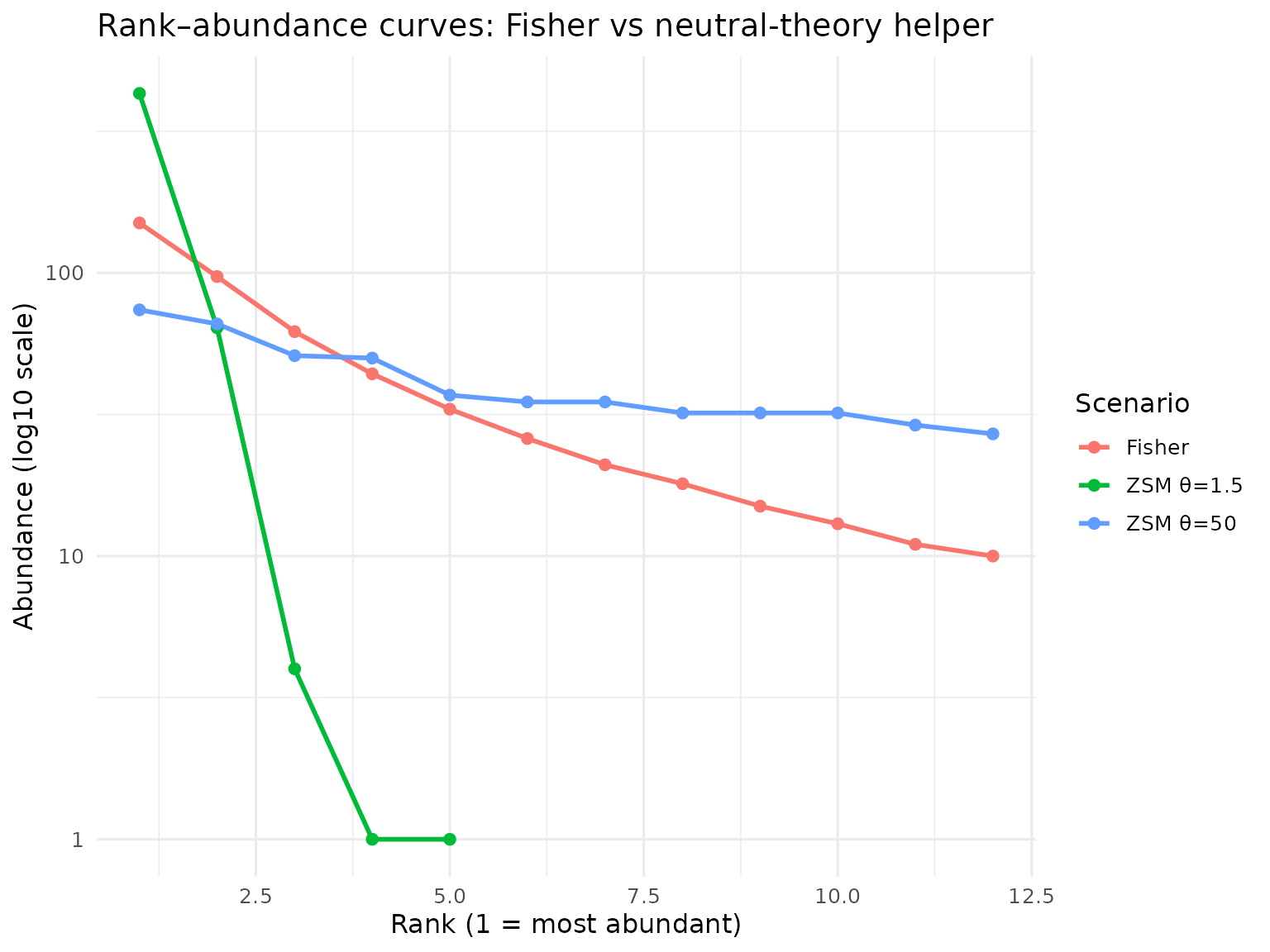

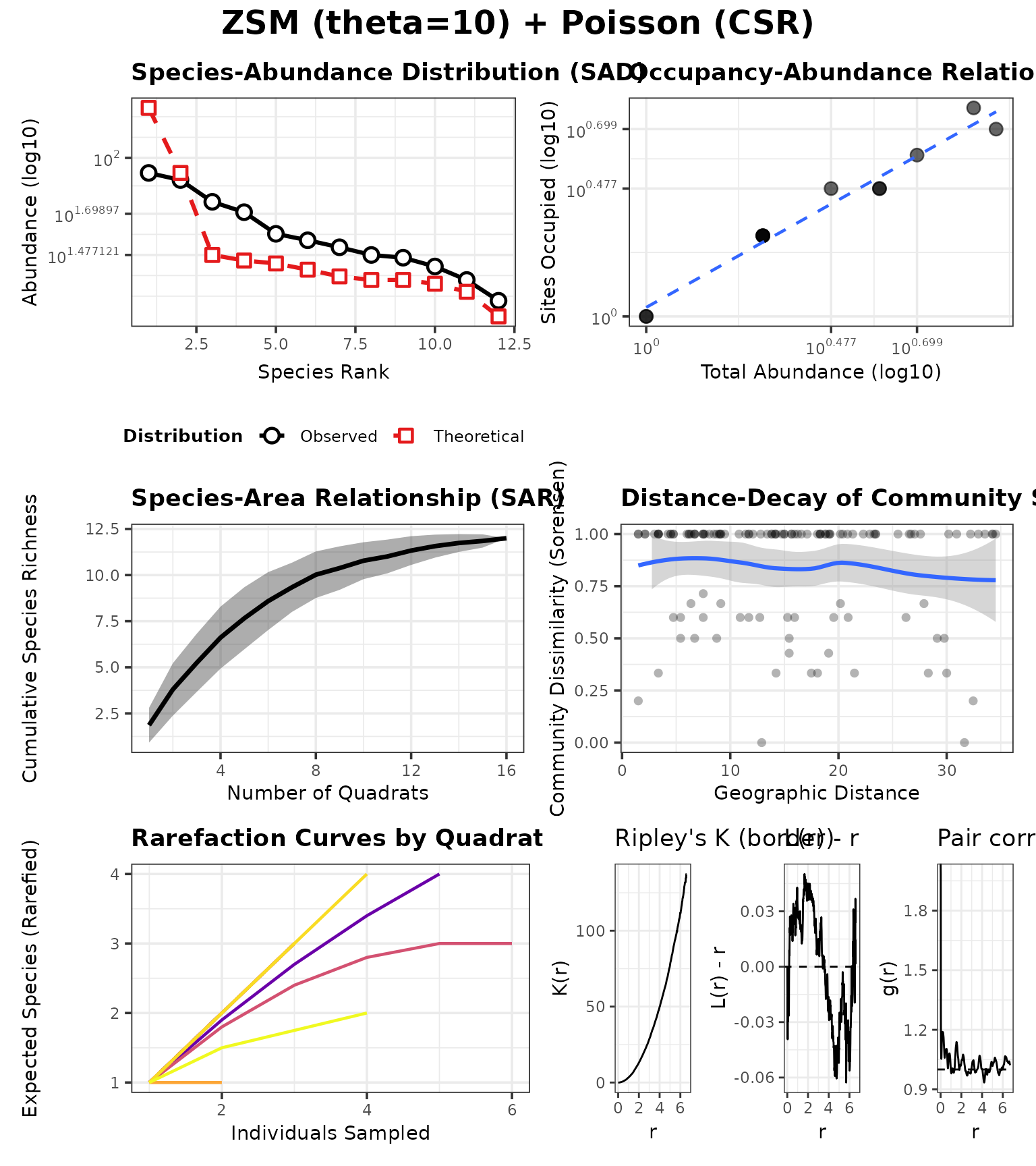
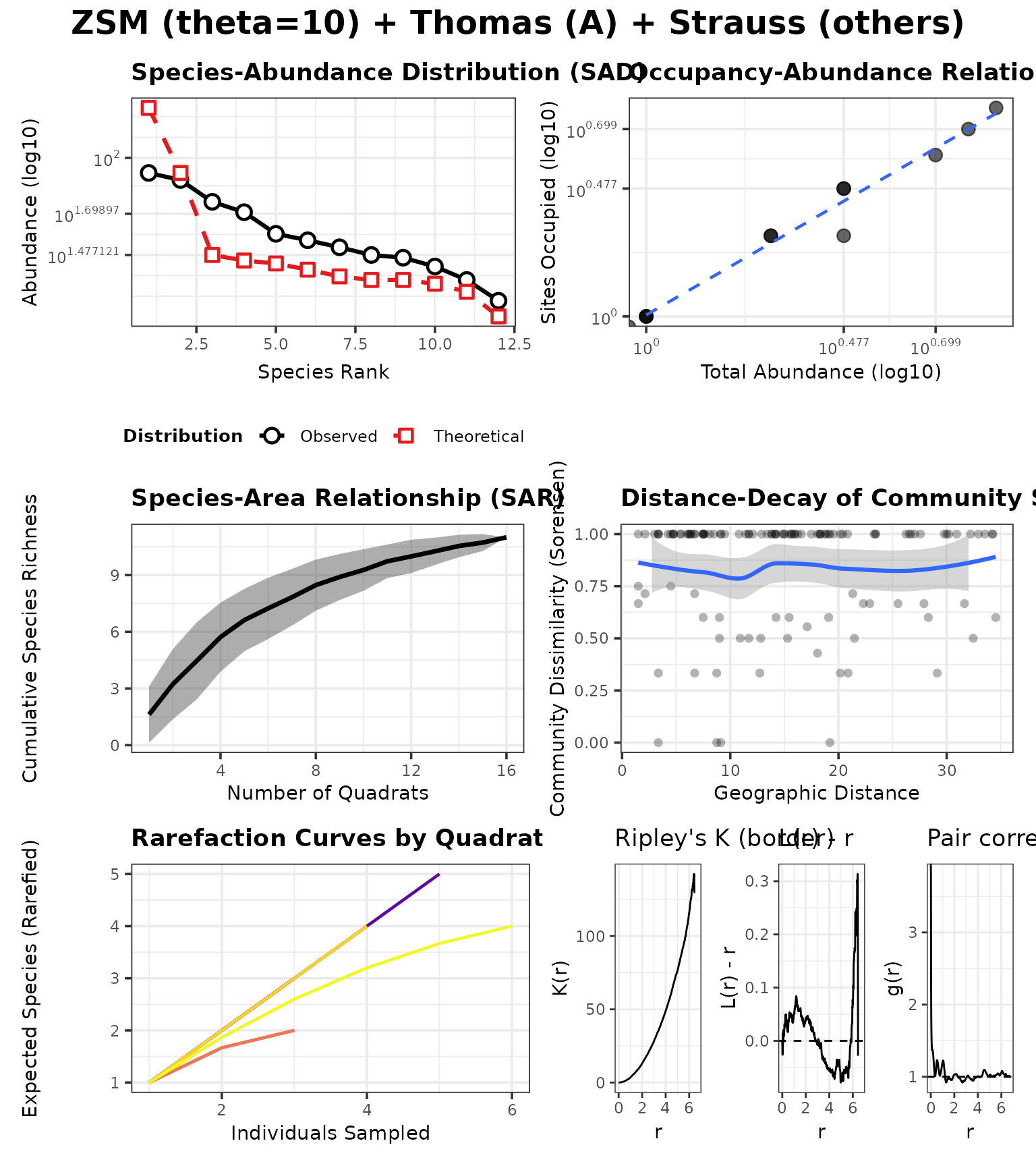
Full advanced panels

case_fisher$panel

case_zlow$panel

case_zhigh$panel

Example B: Spatial differences (distance–decay) under a fixed neutral SAD

Now we fix the SAD model to neutral-theory ZSM and vary only the point-process.

To make the contrast obvious, we choose a strongly structured placement:

Dominant species A: tight Thomas clustering (many offspring, small sigma)
Other species: strong Strauss inhibition (repulsion)

P_neutral <- P0
P_neutral$SAD_MODEL <- "zsm"
P_neutral$ZSM_THETA <- 10
P_neutral$ZSM_M <- NA_real_

# CSR baseline
P_neutral_pois <- P_neutral
P_neutral_pois$SPATIAL_PROCESS_A <- "poisson"
P_neutral_pois$SPATIAL_PROCESS_OTHERS <- "poisson"

# Strong spatial structure
P_neutral_struct <- P_neutral
P_neutral_struct$SPATIAL_PROCESS_A <- "thomas"
P_neutral_struct$A_PARENT_INTENSITY <- NA
P_neutral_struct$A_MEAN_OFFSPRING <- 25
P_neutral_struct$A_CLUSTER_SCALE <- 0.45

P_neutral_struct$SPATIAL_PROCESS_OTHERS <- "strauss"
P_neutral_struct$OTHERS_R <- 1.2
P_neutral_struct$OTHERS_STRAUSS_GAMMA <- 0.15

case_neutral_pois   <- run_case(P_neutral_pois,   "ZSM (theta=10) + Poisson (CSR)")
case_neutral_struct <- run_case(P_neutral_struct, "ZSM (theta=10) + Thomas (A) + Strauss (others)")

Distance–decay (overlay)

dd_all <- rbind(
  decay_df(case_neutral_pois$res,   "Poisson"),
  decay_df(case_neutral_struct$res, "Thomas + Strauss")
)

ggplot(dd_all, aes(Distance, Dissimilarity, colour = Scenario)) +
  geom_point(alpha = 0.25) +
  geom_smooth(se = FALSE, linewidth = 1.2, method = "loess", span = 0.75) +
  labs(
    title = "Distance–decay under the same neutral SAD",
    subtitle = "Spatial structure changes turnover with distance; SAD model is held constant",
    x = "Inter-quadrat distance",
    y = "Community dissimilarity (Bray–Curtis on presence/absence)"
  ) +
  theme_minimal(base_size = 12)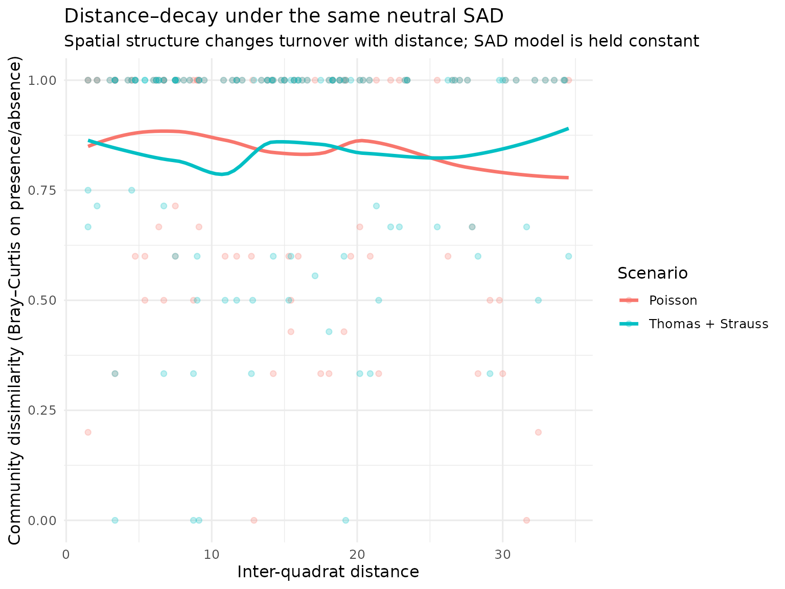

Full advanced panels

case_neutral_pois$panel

case_neutral_struct$panel

Example C: Model families (neutral_hubbell_like vs hybrid)

Here we switch from point-process assembly to the high-level family layer.

P_family <- P0
P_family$N_INDIVIDUALS <- 400
P_family$SAD_MODEL <- "zsm"
P_family$ZSM_THETA <- 12

P_family$GRADIENT_SPECIES <- c("A", "B", "C", "D")
P_family$GRADIENT_ASSIGNMENTS <- c("temperature", "temperature", "elevation", "rainfall")
P_family$GRADIENT_OPTIMA <- c(A = 0.25, B = 0.70, C = 0.55, D = 0.60)
P_family$GRADIENT_TOLERANCE <- c(A = 0.12, B = 0.12, C = 0.16, D = 0.14)

P_hubbell <- P_family
P_hubbell$MODEL_FAMILY <- "neutral_hubbell_like"
P_hubbell$NEUTRAL_M <- 0.08
P_hubbell$DISPERSAL_KERNEL <- "gaussian"
P_hubbell$DISPERSAL_SCALE <- 0.55

P_hybrid <- P_hubbell
P_hybrid$MODEL_FAMILY <- "hybrid"
P_hybrid$HYBRID_ENV_WEIGHT <- 1.3

case_hubbell <- run_case(P_hubbell, "MODEL_FAMILY = neutral_hubbell_like")
case_hybrid  <- run_case(P_hybrid,  "MODEL_FAMILY = hybrid")

dd_family <- rbind(
  decay_df(case_hubbell$res, "neutral_hubbell_like"),
  decay_df(case_hybrid$res,  "hybrid")
)

ggplot(dd_family, aes(Distance, Dissimilarity, colour = Scenario)) +
  geom_point(alpha = 0.25) +
  geom_smooth(se = FALSE, linewidth = 1.2, method = "loess", span = 0.75) +
  labs(
    title = "Model-family comparison",
    subtitle = "Hybrid combines neutral recruitment with environmental sorting",
    x = "Inter-quadrat distance",
    y = "Community dissimilarity (Bray–Curtis on presence/absence)"
  ) +
  theme_minimal(base_size = 12)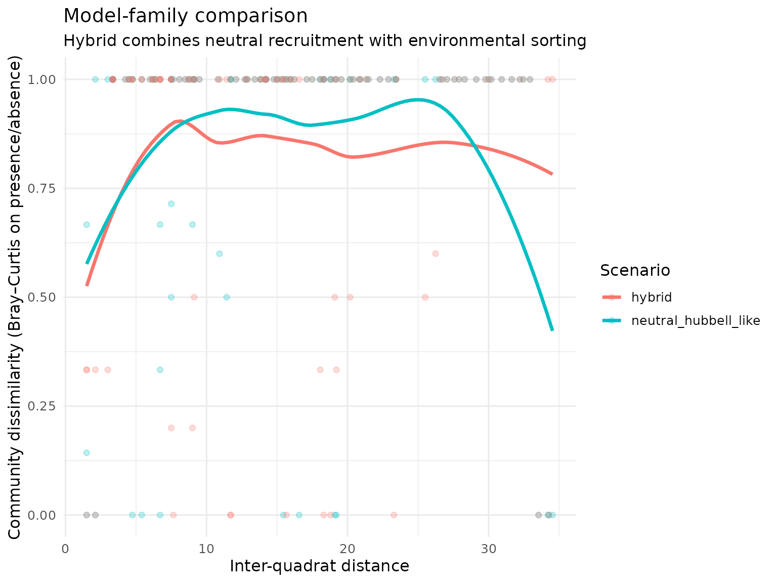

Notes / tips

Use MODEL_FAMILY = "manual" when you want full low-level control.
Use MODEL_FAMILY = "neutral_hubbell_like" or "hybrid" when you want dispersal-driven structure to emerge from recruitment.
For Doubs-style/seaweed-style constrained gradients, set DOMAIN_TYPE = "network" or "coastline" and use DISTANCE_METRIC = "along_path".
You can replace synthetic raster fields by supplying ENV_COVARIATES_FILE (section/node-level covariates with x,y plus environmental columns).
If the distance–decay looks noisy, increase N_QUADRATS and/or reduce quadrat size.
For pedagogy, it helps to vary one knob at a time (SAD vs point process), then show how they interact.