spesim: Doubs network method and interpolation workflow
Source:vignettes/spesim-doubs-network-method.Rmd
spesim-doubs-network-method.RmdThis vignette documents, in detail, the Doubs real-data workflow for:
- constructing a directed site network from observed localities,
and
- simulating species composition at unsampled positions between observed sites.
It uses only observed Doubs data from inst/extdata:
-
DoubsSpa.csv(site coordinates), -
DoubsEnv.csv(site-level environment), -
DoubsSpe.csv(site x species abundances).
Method summary
The current method is a linearized network MVP:
- Sites are ordered by an along-river coordinate (
dfsin DoubsEnv). - Edges are created between consecutive ordered sites.
- Edge weight is Euclidean segment length in projected site coordinates.
- Distance-decay along the network uses shortest-path distance over this edge graph.
Interpolation to unsampled sites uses:
-
linear_posbetween 0 and 1 as the 1D route coordinate, - coordinate/environment interpolation along
linear_pos, - inverse-distance weighted (IDW-like) borrowing of observed community structure,
- optional directional bias to favor downstream or upstream influence.
Load and join observed Doubs data
library(spesim)
library(ggplot2)
library(sf)
library(dplyr)

pkg_file <- function(subpath, folder = "extdata") {
  p_inst <- system.file(folder, subpath, package = "spesim")
  if (nzchar(p_inst) && file.exists(p_inst)) return(p_inst)
  cand <- c(file.path("inst", folder, subpath), file.path("..", "inst", folder, subpath))
  for (p in cand) if (file.exists(p)) return(p)
  stop("Could not find: ", subpath)
}

read_with_site <- function(path) {
  x <- read.csv(path, check.names = FALSE)
  if ("" %in% names(x)) names(x)[names(x) == ""] <- "site"
  x
}

doubs_spa <- read_with_site(pkg_file("DoubsSpa.csv"))
doubs_env <- read_with_site(pkg_file("DoubsEnv.csv"))
doubs_spe <- read_with_site(pkg_file("DoubsSpe.csv"))

doubs <- merge(doubs_spa, doubs_env, by = "site", sort = TRUE)
names(doubs)[names(doubs) == "X"] <- "x"
names(doubs)[names(doubs) == "Y"] <- "y"
doubs$linear_pos <- (doubs$dfs - min(doubs$dfs)) / (max(doubs$dfs) - min(doubs$dfs))

site_coords_doubs <- doubs[, c("site", "x", "y", "linear_pos")]
site_coords_doubs$site <- as.character(site_coords_doubs$site)
doubs_abund <- doubs_spe
names(doubs_abund)[1] <- "site"
doubs_abund$site <- as.character(doubs_abund$site)
doubs_site_env <- doubs[, c("site", "dfs", "alt", "flo", "pH", "nit", "oxy", "bod")]
doubs_site_env$site <- as.character(doubs_site_env$site)
Step 1: Create the network
Construction rule
build_network_edges() creates a chain graph:
- sort sites by
linear_pos(here derived fromdfs), - connect each site to the next one,
- compute edge weight as segment length between coordinates,
- if
directed = TRUE, keep edge direction from low to highlinear_pos.
doubs_edges <- build_network_edges(
  site_coords = site_coords_doubs,
  order_by = "linear_pos",
  directed = TRUE
)

head(doubs_edges, 8)
#>   from to     weight
#> 1    1  2  0.7298829
#> 2    2  3  8.2233893
#> 3    3  4  2.8258921
#> 4    4  5  2.8265613
#> 5    5  6  8.1698045
#> 6    6  7  3.3495171
#> 7    7  8  7.7096670
#> 8    8  9 14.0042711
Plot the network geometry
edge_xy <- doubs_edges |>
  left_join(site_coords_doubs |> select(site, x_from = x, y_from = y), by = c("from" = "site")) |>
  left_join(site_coords_doubs |> select(site, x_to = x, y_to = y), by = c("to" = "site"))

ggplot() +
  geom_path(
    data = site_coords_doubs[order(site_coords_doubs$linear_pos), ],
    aes(x, y),
    linewidth = 0.6,
    colour = "grey55",
    alpha = 0.6
  ) +
  geom_segment(
    data = edge_xy,
    aes(x = x_from, y = y_from, xend = x_to, yend = y_to, colour = weight),
    linewidth = 0.8,
    arrow = grid::arrow(length = grid::unit(1.6, "mm"), type = "closed")
  ) +
  geom_point(data = site_coords_doubs, aes(x, y), size = 2.2, colour = "black") +
  scale_colour_viridis_c(option = "D", end = 0.9) +
  labs(
    title = "Doubs directed site network",
    subtitle = "Edges connect consecutive sites in river-order (linear_pos from dfs)",
    colour = "Edge length"
  ) +
  theme_minimal(base_size = 12)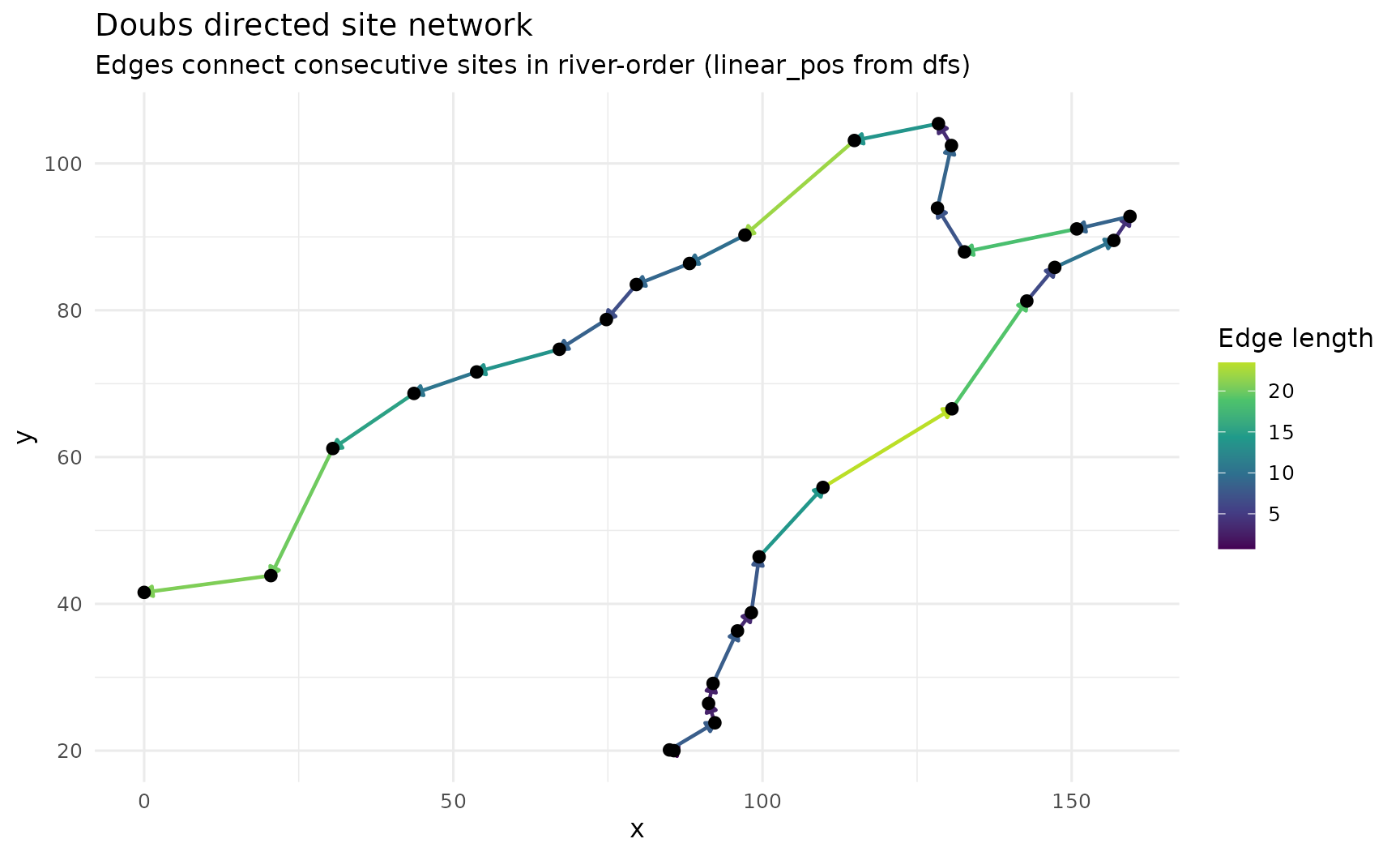
Step 2: Build an observed-data spesim_result (no
simulation yet)
res_doubs_obs <- spesim_from_observed(
  abund_matrix = doubs_abund,
  site_coords = site_coords_doubs,
  site_env = doubs_site_env,
  edges = doubs_edges,
  directed = TRUE
)

res_doubs_obs
#> <spesim_result>
#>   species         : 27
#>   individuals     : 1004
#>   sampling scheme : observed
#>   n_quadrats      : 30
#>   seed            : NA
#>   points          : 1004
#>   quadrats        : 30
This object now supports the standard downstream analyses directly from real data:
- rank-abundance,
- occupancy-abundance,
- species-area accumulation,
- distance-decay,
- rarefaction.
Step 3: Compare Euclidean vs network distance-decay on observed data
dd_eu <- calculate_distance_decay(res_doubs_obs$abund_matrix, res_doubs_obs$site_coords, metric = "euclidean")
dd_net <- calculate_distance_decay(res_doubs_obs$abund_matrix, res_doubs_obs$site_coords, metric = "along_path")

dd <- rbind(
  transform(dd_eu, Metric = "Euclidean"),
  transform(dd_net, Metric = "Network shortest-path")
)

ggplot(dd, aes(Distance, Dissimilarity, colour = Metric)) +
  geom_point(alpha = 0.28) +
  geom_smooth(method = "loess", se = FALSE, span = 0.8, linewidth = 1.1) +
  labs(
    title = "Doubs observed distance-decay: Euclidean vs network distance",
    y = "Bray-Curtis (binary)"
  ) +
  theme_minimal(base_size = 12)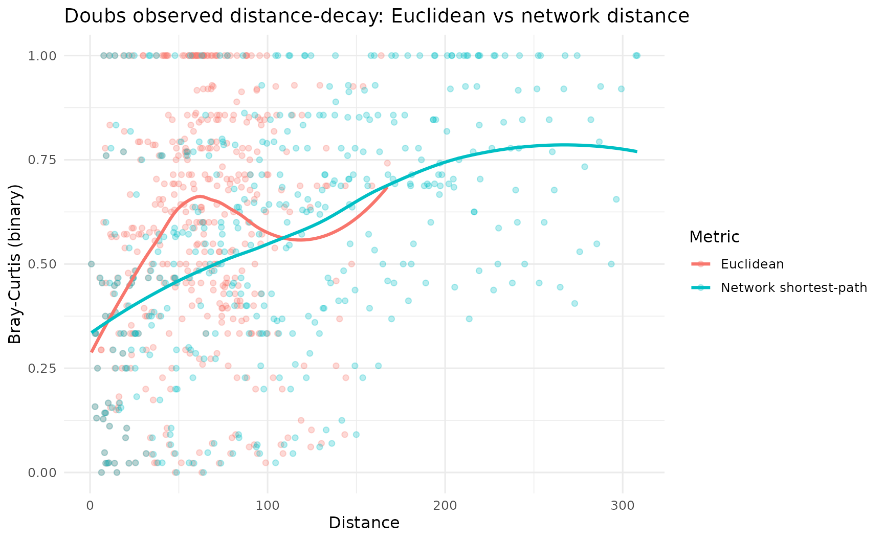
Step 4: Simulate unsampled sites between observed sites
Interpolation model used here
simulate_between_observed() does:
- place new pseudo-sites along the
linear_posaxis between min and max observed positions, - interpolate
x,yand numeric environment along that axis, - estimate species probabilities from observed sites using
inverse-distance weights in
linear_pos, - optionally bias influence direction
(
direction_bias > 0favors downstream influence), - sample pseudo-site abundance vectors with multinomial draws.
doubs_interp <- simulate_between_observed(
  res = res_doubs_obs,
  n_new_sites = 24,
  distance_power = 2,
  direction_bias = 0.35
)

head(doubs_interp$site_coords, 6)
#>       site         x        y linear_pos
#> 1 interp_1  91.29132 26.40179       0.04
#> 2 interp_2  98.05597 38.63867       0.08
#> 3 interp_3 102.12072 48.84766       0.12
#> 4 interp_4 111.41559 56.70384       0.16
#> 5 interp_5 124.66874 63.50927       0.20
#> 6 interp_6 135.57708 72.56192       0.24
head(doubs_interp$abund_matrix[, 1:8], 4)
#>       site Cogo Satr Phph Babl Thth Teso Chna
#> 1 interp_1    0    6    5    3    0    0    0
#> 2 interp_2    0    6    5    4    0    0    0
#> 3 interp_3    0    0    0    1    0    0    0
#> 4 interp_4    0    0    0    2    0    0    0
Plot observed + interpolated sites
ggplot() +
  geom_point(data = res_doubs_obs$site_coords, aes(x, y), size = 2.1, colour = "black") +
  geom_point(data = doubs_interp$site_coords, aes(x, y), size = 1.8, colour = "red", alpha = 0.8) +
  labs(
    title = "Doubs observed (black) and interpolated unsampled sites (red)"
  ) +
  theme_minimal(base_size = 12)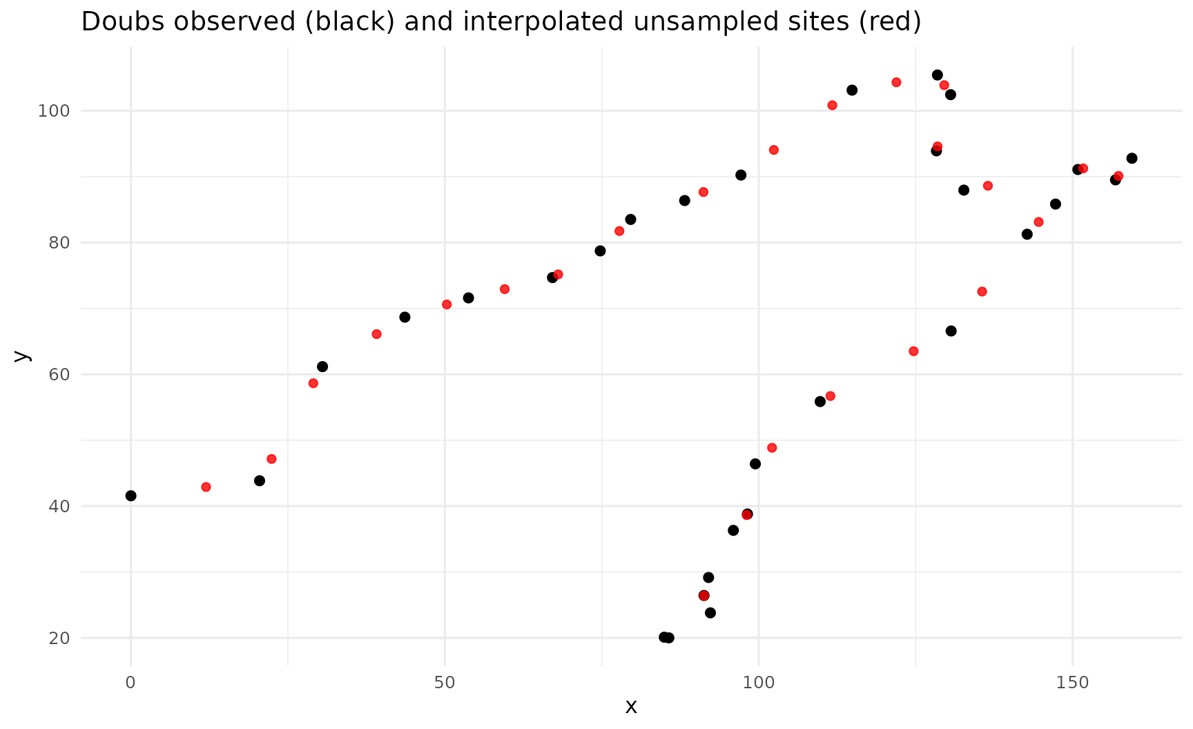
Step 5: Build a spesim_result for interpolated sites
and analyse
res_doubs_interp <- spesim_from_observed(
  abund_matrix = doubs_interp$abund_matrix,
  site_coords = doubs_interp$site_coords,
  site_env = doubs_interp$site_env,
  edges = build_network_edges(doubs_interp$site_coords, order_by = "linear_pos", directed = TRUE),
  directed = TRUE
)

res_doubs_interp
#> <spesim_result>
#>   species         : 27
#>   individuals     : 921
#>   sampling scheme : observed
#>   n_quadrats      : 24
#>   seed            : NA
#>   points          : 921
#>   quadrats        : 24
panel_ready_res <- function(res, max_species = 26L) {
  spp <- setdiff(names(res$abund_matrix), "site")
  if (length(spp) <= max_species) return(res)
  sums <- colSums(res$abund_matrix[, spp, drop = FALSE], na.rm = TRUE)
  keep <- names(sort(sums, decreasing = TRUE))[seq_len(max_species)]
  out <- res
  out$abund_matrix <- cbind(site = res$abund_matrix$site, res$abund_matrix[, keep, drop = FALSE])
  out$species_dist <- res$species_dist[as.character(res$species_dist$species) %in% keep, ]
  out$P$N_SPECIES <- length(keep)
  out
}

generate_advanced_panel(panel_ready_res(res_doubs_obs)) +
  patchwork::plot_annotation(title = "Doubs observed data: advanced panel")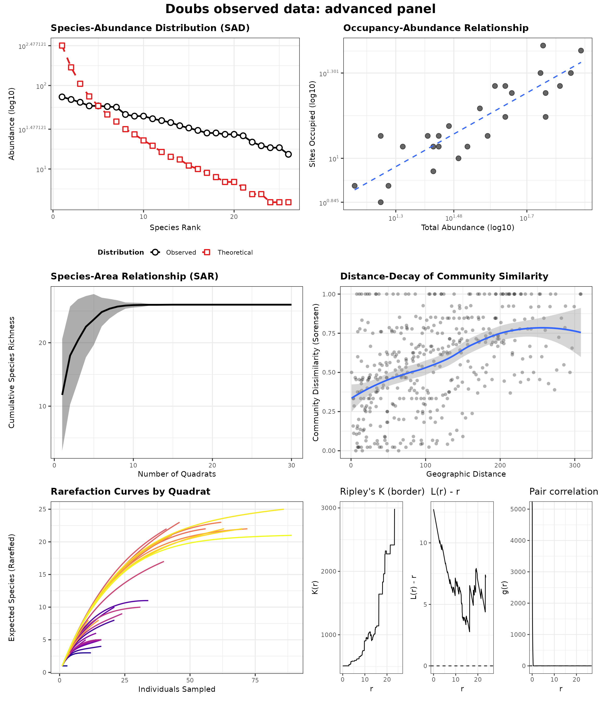
generate_advanced_panel(panel_ready_res(res_doubs_interp)) +
  patchwork::plot_annotation(title = "Doubs interpolated unsampled sites: advanced panel")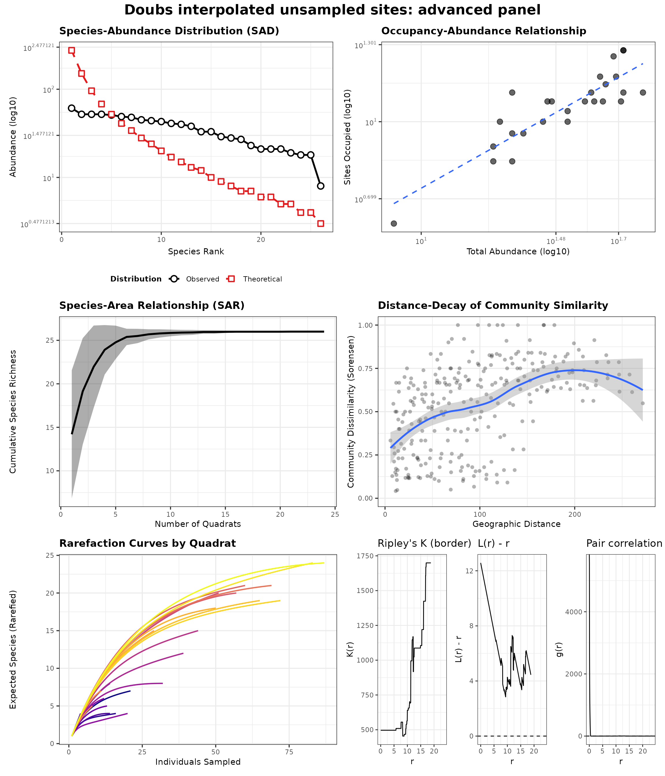
Notes and limitations
- This is still a linearized constrained-landscape approach.
- Network construction here is a chain over ordered observed sites, not yet a full branched river graph with explicit node-edge topology from hydrography.
- Interpolated unsampled communities are model-based pseudo-observations that preserve local observed structure but are not direct measurements.
- The workflow is meant to support method development and sensitivity analysis in realistic spatial constraints while full graph-theoretic routing is added.