spesim recipes: interspecific interactions • spesim

This recipe shows how to specify simple neighbour effects using INTERACTIONS_EDGELIST.

Values:

< 1 suppressive (competition)
> 1 facilitative
= 1 neutral

Baseline without interactions

library(spesim)
#> spesim 0.5.2 loaded - try spesim_run() to generate a simulation.

P <- load_config(system.file("examples/spesim_init_basic.txt", package = "spesim"))
#> ========== INITIALISING SPATIAL SAMPLING SIMULATION ==========
P$N_SPECIES <- 10
P$N_INDIVIDUALS <- 2000
P$ADVANCED_ANALYSIS <- FALSE

# Turn interactions off
P$INTERACTION_RADIUS <- 0
P$INTERACTIONS_EDGELIST <- NULL

set.seed(P$SEED)
res0 <- spesim_run(P, write_outputs = FALSE, seed = P$SEED, interactions_print = FALSE)
#> spesim: running simulation
#> Note: no non-1 interactions for species: A, B, C, D, E, F, G, H, I, J.
plot_spatial_sampling(res0$domain, res0$species_dist, res0$quadrats, res0$P)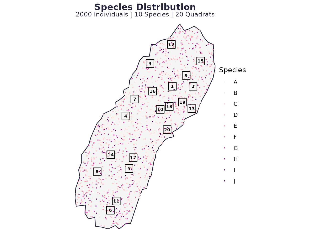

Add a few directed interaction rules

Here, species A suppresses B..D locally, and species C facilitates A.

P2 <- P
P2$INTERACTION_RADIUS <- 2
P2$INTERACTIONS_EDGELIST <- c(
  "A,B-D,0.7",
  "C,A,1.3"
)

res1 <- spesim_run(P2, write_outputs = FALSE, seed = P2$SEED, interactions_print = TRUE)
#> spesim: running simulation
#> Note: no non-1 interactions for species: E, F, G, H, I, J.
#> ---- Interactions Summary ----
#> Species: 10 (A..J)
#> Radius : 2
#> Non-1 entries: 4 (4.0% of 100)
#> Asymmetry (mean |M - t(M)|): 0.024
#> 
#> Matrix ('.' = 1):
#>   A   B   C   D   E F G H I J
#> A .   0.7 0.7 0.7 . . . . . .
#> B .   .   .   .   . . . . . .
#> C 1.3 .   .   .   . . . . . .
#> D .   .   .   .   . . . . . .
#> E .   .   .   .   . . . . . .
#> F .   .   .   .   . . . . . .
#> G .   .   .   .   . . . . . .
#> H .   .   .   .   . . . . . .
#> I .   .   .   .   . . . . . .
#> J .   .   .   .   . . . . . .
#> 
#> Non-1 entries (sorted by |value-1|):
#>  focal neighbor value
#>      A        B   0.7
#>      A        C   0.7
#>      A        D   0.7
#>      C        A   1.3
#> ------------------------------

# Visualise the outcome
plot_spatial_sampling(res1$domain, res1$species_dist, res1$quadrats, res1$P)

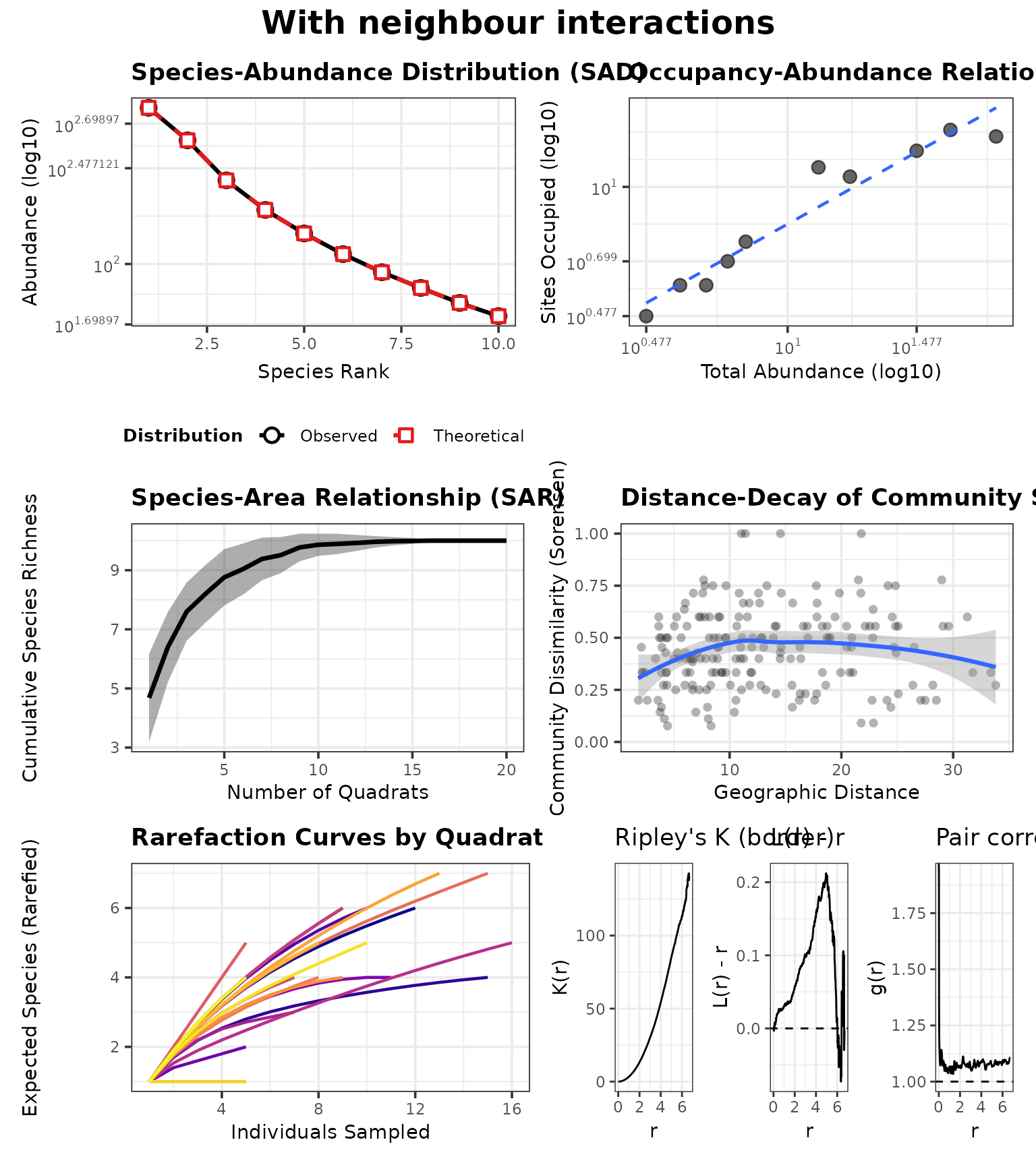
Consequences in the advanced analysis panel

Neighbour effects can change co-occurrence patterns and local abundance, which in turn changes what you observe in quadrats.

In ecological terms, competition (coefficients < 1) can create spatial segregation and reduce local richness in neighbourhoods dominated by a strong competitor, while facilitation (> 1) can increase local co-occurrence.

In the advanced panel, interaction effects can manifest as:

shifts in occupancy–abundance (suppressed species become rarer and occupy fewer sites),
changes in distance–decay (if interactions amplify patchiness),
and altered rarefaction curves (effective evenness/richness per site).

panel0 <- generate_advanced_panel(res0) + patchwork::plot_annotation(title = "Baseline: no interactions")
panel1 <- generate_advanced_panel(res1) + patchwork::plot_annotation(title = "With neighbour interactions")

panel0
#> `geom_smooth()` using formula = 'y ~ x'
#> `geom_smooth()` using formula = 'y ~ x'
#> Warning: Removed 1 row containing missing values or values outside the scale range
#> (`geom_line()`).
#> Removed 1 row containing missing values or values outside the scale range
#> (`geom_line()`).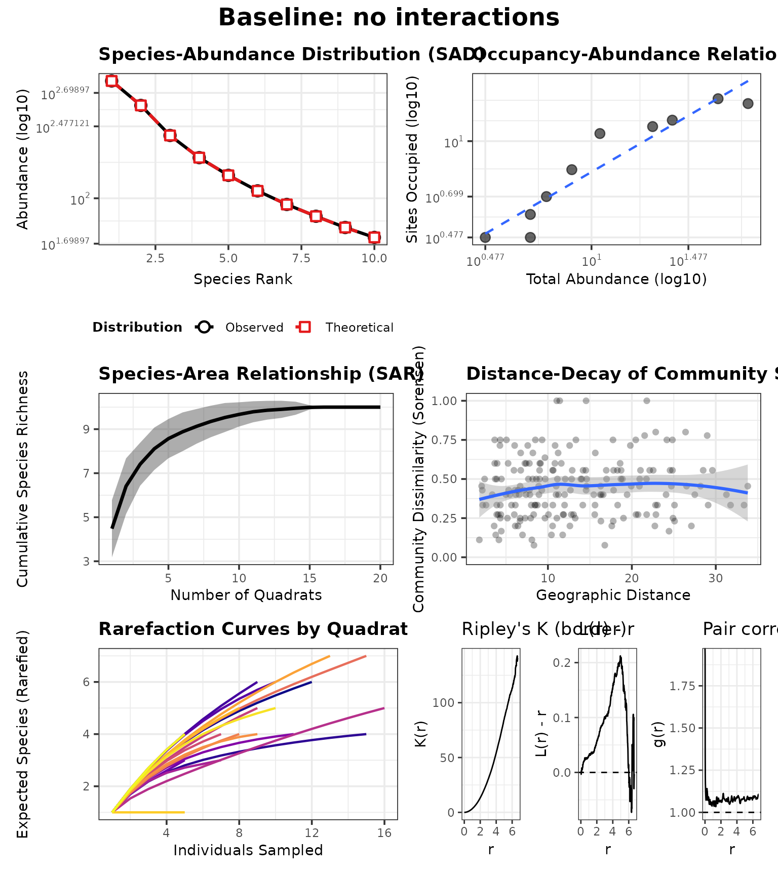

panel1
#> `geom_smooth()` using formula = 'y ~ x'
#> `geom_smooth()` using formula = 'y ~ x'
#> Warning: Removed 1 row containing missing values or values outside the scale range
#> (`geom_line()`).
#> Removed 1 row containing missing values or values outside the scale range
#> (`geom_line()`).

Notes

Rules are directed (A -> B need not equal B -> A).
The global INTERACTION_RADIUS controls the neighbourhood size.
Keep INTERACTION_RADIUS = 0 to disable the modifier.