spesim recipes: environmental gradients • spesim

This short recipe shows how to turn environmental filtering on and off, and how to change optima/tolerances for gradient-responsive species.

Minimal run without special gradients

library(spesim)
#> spesim 0.5.2 loaded - try spesim_run() to generate a simulation.

P <- load_config(system.file("examples/spesim_init_basic.txt", package = "spesim"))
#> ========== INITIALISING SPATIAL SAMPLING SIMULATION ==========
P$N_SPECIES <- 10
P$N_INDIVIDUALS <- 1200
P$ADVANCED_ANALYSIS <- FALSE

set.seed(P$SEED)
res0 <- spesim_run(P, write_outputs = FALSE, seed = P$SEED)
#> spesim: running simulation
#> Note: no non-1 interactions for species: A, B, C, D, E, F, G, H, I, J.
#> ---- Interactions Summary ----
#> Species: 10 (A..J)
#> Radius : 0
#> Non-1 entries: 0 (0.0% of 100)
#> 
#> Matrix ('.' = 1):
#>   A B C D E F G H I J
#> A . . . . . . . . . .
#> B . . . . . . . . . .
#> C . . . . . . . . . .
#> D . . . . . . . . . .
#> E . . . . . . . . . .
#> F . . . . . . . . . .
#> G . . . . . . . . . .
#> H . . . . . . . . . .
#> I . . . . . . . . . .
#> J . . . . . . . . . .
#> ------------------------------
plot_spatial_sampling(res0$domain, res0$species_dist, res0$quadrats, res0$P)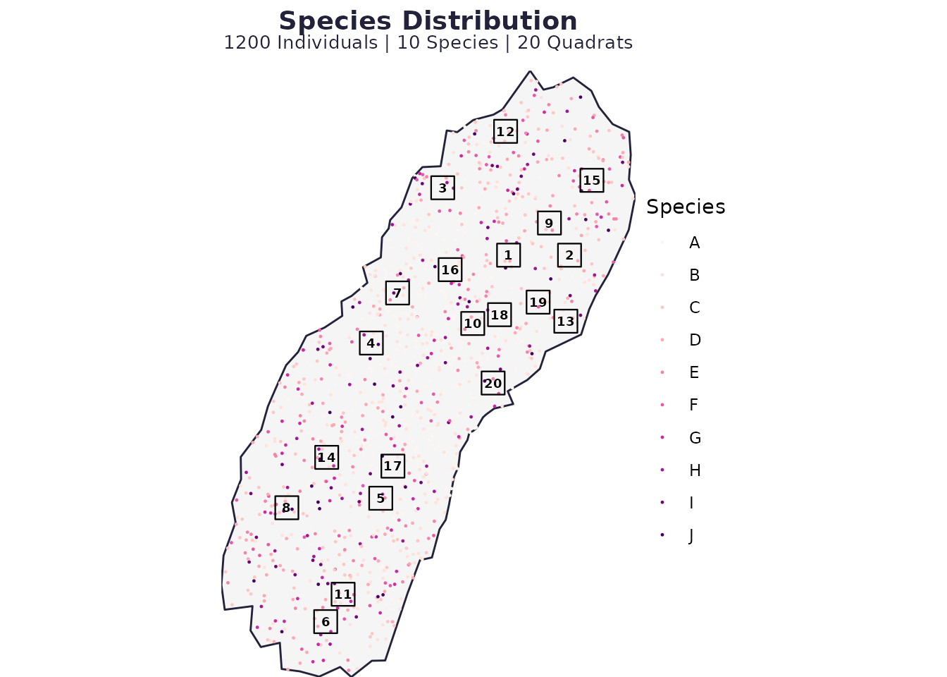

Make a few species respond strongly to a gradient

Here we keep everything else the same but make the temperature-responsive species prefer warmer areas by shifting their optimum upward and tightening their tolerance.

P2 <- P

# A and B respond to temperature; C to elevation; D to rainfall (from the example init)
# Push temperature optimum to the warm end and make the response sharper
P2$GRADIENT_OPTIMA <- c(temperature = 0.80, elevation = 0.50, rainfall = 0.50)
P2$GRADIENT_TOLERANCE <- c(temperature = 0.07, elevation = 0.12, rainfall = 0.12)

res1 <- spesim_run(P2, write_outputs = FALSE, seed = P2$SEED)
#> spesim: running simulation
#> Note: no non-1 interactions for species: A, B, C, D, E, F, G, H, I, J.
#> ---- Interactions Summary ----
#> Species: 10 (A..J)
#> Radius : 0
#> Non-1 entries: 0 (0.0% of 100)
#> 
#> Matrix ('.' = 1):
#>   A B C D E F G H I J
#> A . . . . . . . . . .
#> B . . . . . . . . . .
#> C . . . . . . . . . .
#> D . . . . . . . . . .
#> E . . . . . . . . . .
#> F . . . . . . . . . .
#> G . . . . . . . . . .
#> H . . . . . . . . . .
#> I . . . . . . . . . .
#> J . . . . . . . . . .
#> ------------------------------

p1 <- plot_spatial_sampling(res1$domain, res1$species_dist, res1$quadrats, res1$P)

# Show the underlying temperature field
p2 <- plot_spatial_sampling(
  res1$domain, res1$species_dist, res1$quadrats, res1$P,
  show_gradient = TRUE,
  env_gradients = res1$env_gradients,
  gradient_type = "temperature_C"
)

p1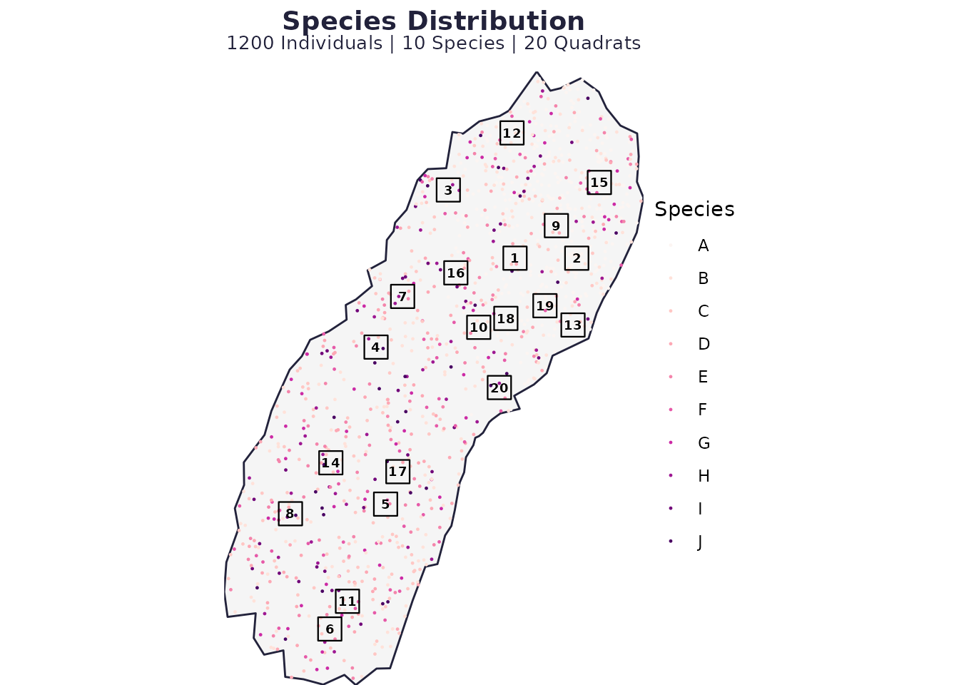

p2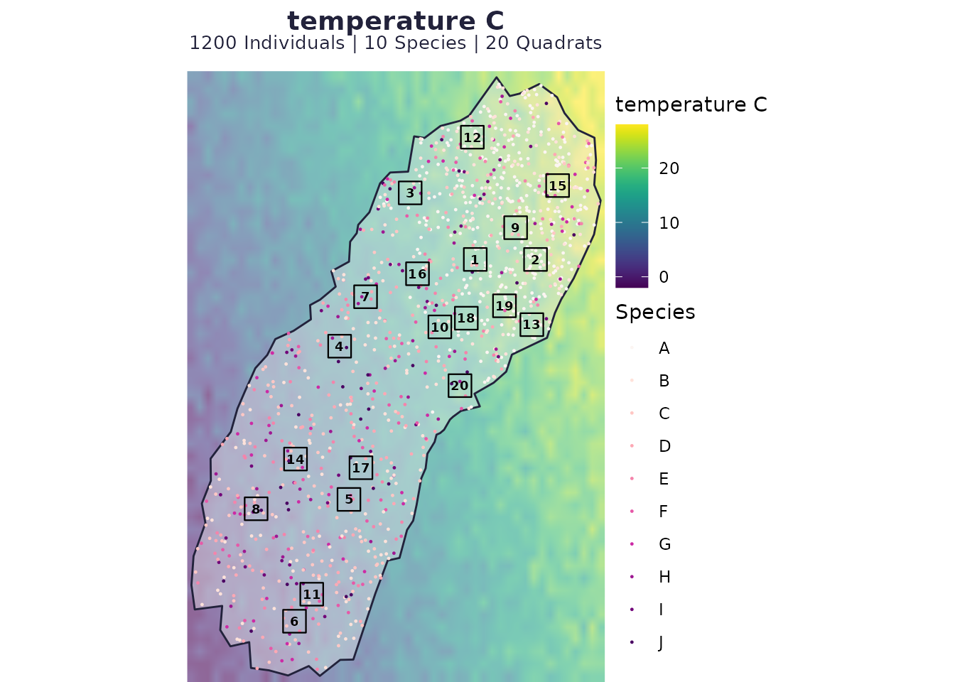

Consequences in the advanced analysis panel

Environmental filtering typically increases spatial turnover (beta diversity) when species have different optima along a gradient. In the advanced panel this often shows up as:

a stronger distance–decay signal (dissimilarity increases with distance),
a steeper species–area curve (more quadrats needed to capture gamma diversity),
and changes in occupancy–abundance patterns (specialists can be abundant but occupy fewer sites).

This is consistent with classic niche-based theory: species are sorted along environmental axes (e.g. temperature), so communities separated along the axis share fewer species.

# Compare advanced panels: baseline vs stronger filtering
panel0 <- generate_advanced_panel(res0) + patchwork::plot_annotation(title = "Baseline: weak/default filtering")
panel1 <- generate_advanced_panel(res1) + patchwork::plot_annotation(title = "Stronger temperature filtering")

panel0
#> `geom_smooth()` using formula = 'y ~ x'
#> `geom_smooth()` using formula = 'y ~ x'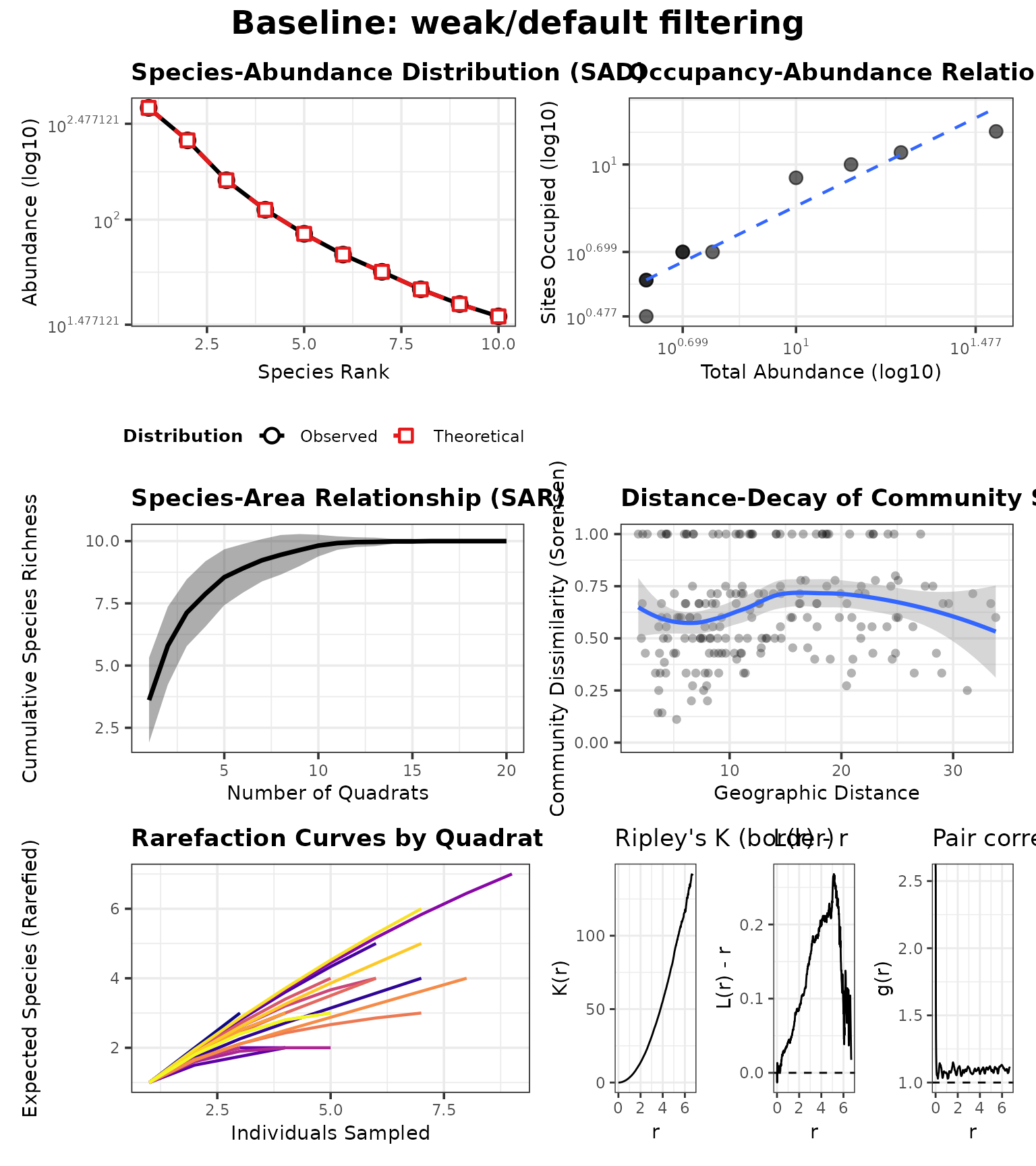

panel1
#> `geom_smooth()` using formula = 'y ~ x'
#> `geom_smooth()` using formula = 'y ~ x'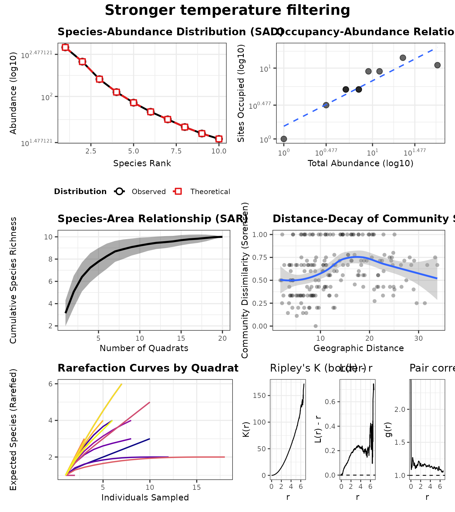

Tip: reproducibility

If you want exact repeatability for gradient-driven patterns, set the seed (via init file or P$SEED) and call set.seed() before running.