spesim: real-world constrained landscapes (Doubs + seaweed)
Source:vignettes/spesim-real-world-landscapes.Rmd
spesim-real-world-landscapes.RmdThis vignette shows how to use real-world coordinates and covariates
from inst/extdata:
- Doubs river data:
DoubsSpa.csv,DoubsEnv.csv,DoubsSpe.csv - Seaweed coastline data:
SeaweedSpa.csv,SeaweedEnv.csv,SeaweedSpe.csv
It also uses pre-merged covariate files shipped in the package:
DoubsCovariates.csvSeaweedCovariates.csv
Limitation note
This is a linearized constrained-landscape MVP, not yet a full graph-theoretic river-network engine (no explicit edge/node topology or true network shortest-path over branches yet).
Helpers
library(spesim)
library(ggplot2)
library(sf)

read_with_site <- function(path) {
  x <- read.csv(path, check.names = FALSE)
  if ("" %in% names(x)) names(x)[names(x) == ""] <- "site"
  x
}

pkg_file <- function(subpath, folder = c("extdata", "examples")) {
  folder <- match.arg(folder)
  p_installed <- system.file(folder, subpath, package = "spesim")
  if (nzchar(p_installed) && file.exists(p_installed)) return(p_installed)
  candidates <- c(
    file.path("inst", folder, subpath),
    file.path("..", "inst", folder, subpath)
  )
  for (p_local in candidates) {
    if (file.exists(p_local)) return(p_local)
  }
  stop("Could not find file: ", subpath, " in ", folder)
}

make_domain_from_xy <- function(df, buffer_frac = 0.06) {
  pts <- st_as_sf(df, coords = c("x", "y"), crs = NA)
  hull <- st_convex_hull(st_union(pts))
  bb <- st_bbox(hull)
  d <- sqrt((bb["xmax"] - bb["xmin"])^2 + (bb["ymax"] - bb["ymin"])^2)
  st_as_sf(st_buffer(hull, d * buffer_frac))
}

build_linear_pos <- function(x) {
  rng <- range(x, na.rm = TRUE)
  den <- rng[2] - rng[1]
  if (!is.finite(den) || den == 0) den <- 1
  pmax(0, pmin(1, (x - rng[1]) / den))
}

panel_ready_res <- function(res, max_species = 26L) {
  spp <- setdiff(names(res$abund_matrix), "site")
  if (length(spp) <= max_species) return(res)
  sums <- colSums(res$abund_matrix[, spp, drop = FALSE], na.rm = TRUE)
  keep <- names(sort(sums, decreasing = TRUE))[seq_len(max_species)]
  out <- res
  out$abund_matrix <- cbind(site = res$abund_matrix$site, res$abund_matrix[, keep, drop = FALSE])
  out$species_dist <- res$species_dist[as.character(res$species_dist$species) %in% keep, ]
  out$P$N_SPECIES <- length(keep)
  out
}
1) Tie Doubs environmental data to real coordinates
DoubsSpa.csv provides site coordinates (X,
Y). DoubsEnv.csv provides site-level
environmental variables. We join by site ID.
doubs_spa <- read_with_site(pkg_file("DoubsSpa.csv", "extdata"))
doubs_env <- read_with_site(pkg_file("DoubsEnv.csv", "extdata"))
doubs_spe <- read_with_site(pkg_file("DoubsSpe.csv", "extdata"))

doubs <- merge(doubs_spa, doubs_env, by = "site", sort = TRUE)
names(doubs)[names(doubs) == "X"] <- "x"
names(doubs)[names(doubs) == "Y"] <- "y"
doubs$linear_pos <- build_linear_pos(doubs$dfs)

ggplot(doubs, aes(x, y, colour = dfs)) +
  geom_point(size = 2.3) +
  geom_path(alpha = 0.45) +
  labs(
    title = "Doubs sites (from DoubsSpa.csv)",
    subtitle = "Points connected in river-km order (dfs)",
    colour = "dfs"
  ) +
  theme_minimal(base_size = 12)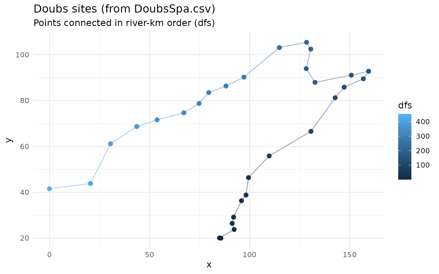
Observed distance-decay from Doubs species data
doubs_abund <- doubs_spe
names(doubs_abund)[1] <- "site"
site_coords_doubs <- doubs[, c("site", "x", "y", "linear_pos")]
doubs_edges <- build_network_edges(site_coords_doubs, order_by = "linear_pos", directed = TRUE)

res_doubs_obs <- spesim_from_observed(
  abund_matrix = doubs_abund,
  site_coords = site_coords_doubs,
  site_env = doubs[, c("site", "dfs", "alt", "flo", "pH", "nit", "oxy")],
  edges = doubs_edges,
  directed = TRUE
)

dd_doubs_eu <- calculate_distance_decay(res_doubs_obs$abund_matrix, res_doubs_obs$site_coords, metric = "euclidean")
dd_doubs_ap <- calculate_distance_decay(res_doubs_obs$abund_matrix, res_doubs_obs$site_coords, metric = "along_path")

dd_doubs <- rbind(
  transform(dd_doubs_eu, Metric = "Euclidean"),
  transform(dd_doubs_ap, Metric = "Along-path")
)

ggplot(dd_doubs, aes(Distance, Dissimilarity, colour = Metric)) +
  geom_point(alpha = 0.25) +
  geom_smooth(se = FALSE, method = "loess", span = 0.8, linewidth = 1.1) +
  labs(title = "Doubs observed distance-decay", y = "Bray-Curtis (binary)") +
  theme_minimal(base_size = 12)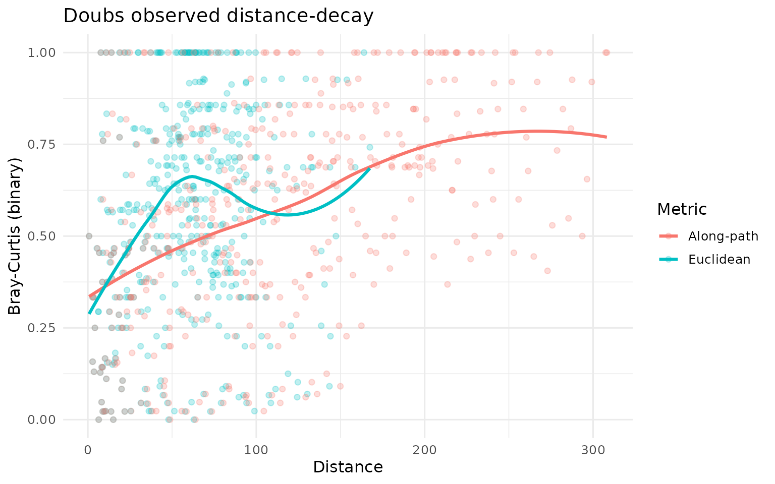
Interpolate unsampled Doubs sites along the network
doubs_interp <- simulate_between_observed(
  res_doubs_obs,
  n_new_sites = 20,
  direction_bias = 0.4
)

ggplot() +
  geom_point(data = res_doubs_obs$site_coords, aes(x, y), color = "black", size = 2) +
  geom_point(data = doubs_interp$site_coords, aes(x, y), color = "red", size = 1.7, alpha = 0.8) +
  labs(title = "Doubs observed sites (black) + interpolated unsampled sites (red)") +
  theme_minimal(base_size = 12)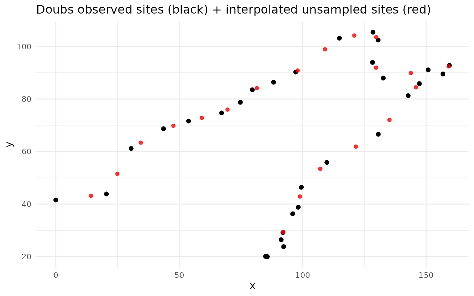
3) Seaweed coastline: real coordinates and covariates
sea_spa <- read.csv(pkg_file("SeaweedSpa.csv", "extdata"), check.names = FALSE)
sea_env <- read_with_site(pkg_file("SeaweedEnv.csv", "extdata"))
sea_spe <- read_with_site(pkg_file("SeaweedSpe.csv", "extdata"))

sea <- transform(sea_spa, site = seq_len(nrow(sea_spa)), x = Longitude, y = Latitude)
sea <- merge(sea[, c("site", "x", "y")], sea_env, by = "site", sort = TRUE)
sea$linear_pos <- build_linear_pos(seq_len(nrow(sea)))

ggplot(sea, aes(x, y, colour = summerMean)) +
  geom_point(size = 2.1) +
  geom_path(alpha = 0.4) +
  labs(title = "Seaweed sections (real coordinates)", colour = "summerMean") +
  theme_minimal(base_size = 12)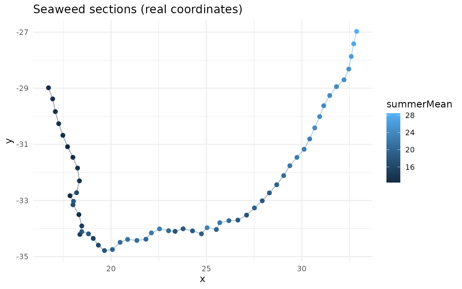
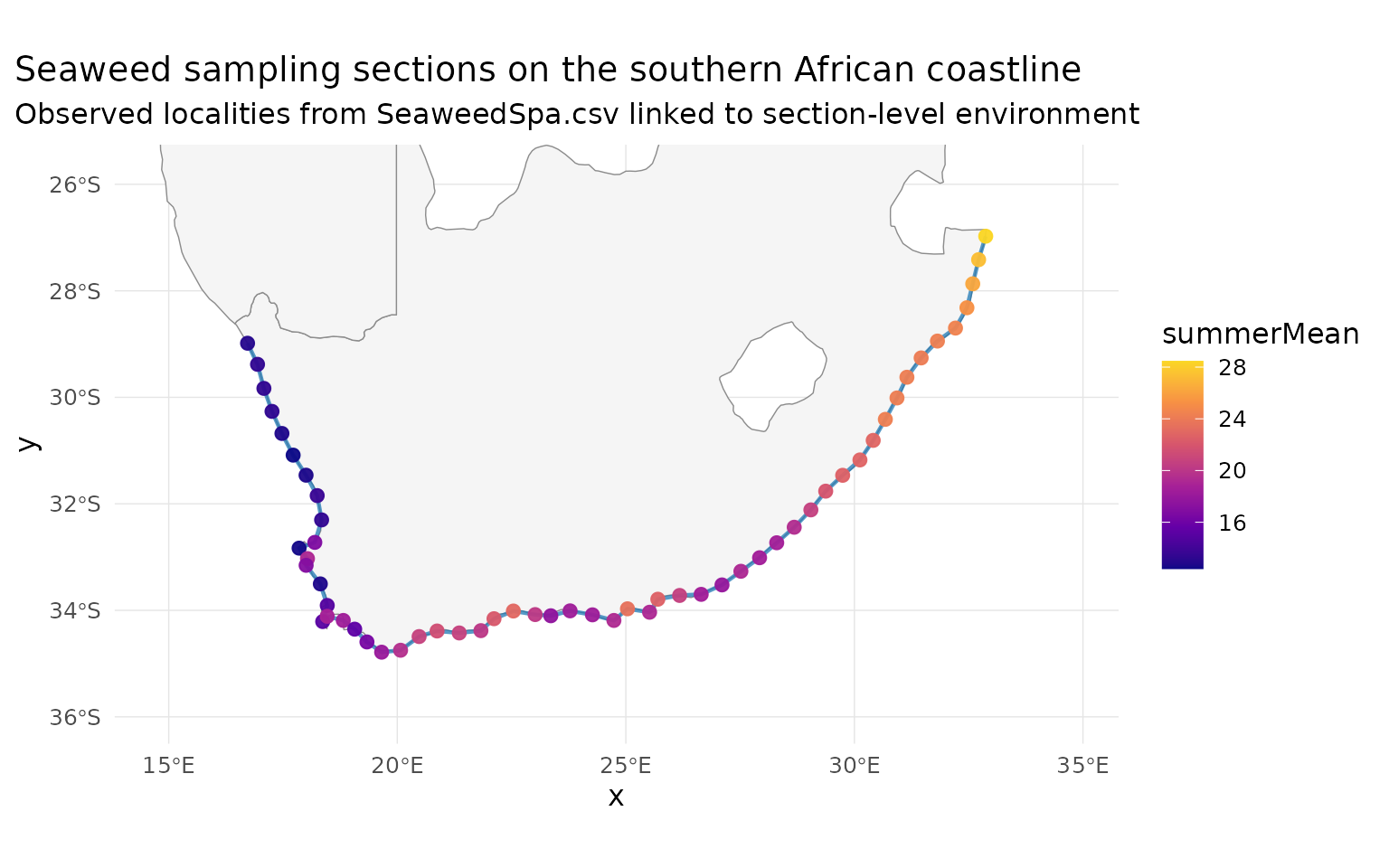
Seaweed sites on a regional basemap (rnaturalearth)
# NOTE: rnaturalearth::ne_countries() will attempt to install rnaturalearthdata
# if it is missing (and this can fail in CI). We therefore require both.
if (requireNamespace("rnaturalearth", quietly = TRUE) &&
    requireNamespace("rnaturalearthdata", quietly = TRUE)) {
  coast_region <- rnaturalearth::ne_countries(
    scale = "medium",
    country = c("South Africa", "Namibia"),
    returnclass = "sf"
  )

  sea_sf <- st_as_sf(sea, coords = c("x", "y"), crs = 4326)
  bb <- st_bbox(sea_sf)
  x_pad <- (bb$xmax - bb$xmin) * 0.18
  y_pad <- (bb$ymax - bb$ymin) * 0.22

  ggplot() +
    geom_sf(data = coast_region, fill = "grey96", colour = "grey55", linewidth = 0.25) +
    geom_path(
      data = sea[order(sea$linear_pos), ],
      aes(x = x, y = y),
      colour = "#1f78b4",
      linewidth = 0.8,
      alpha = 0.75
    ) +
    geom_point(
      data = sea,
      aes(x = x, y = y, colour = summerMean),
      size = 2.2,
      alpha = 0.95
    ) +
    coord_sf(
      xlim = c(bb$xmin - x_pad, bb$xmax + x_pad),
      ylim = c(bb$ymin - y_pad, bb$ymax + y_pad),
      expand = FALSE
    ) +
    scale_colour_viridis_c(option = "C", end = 0.92, name = "summerMean") +
    labs(
      title = "Seaweed sampling sections on the southern African coastline",
      subtitle = "Observed localities from SeaweedSpa.csv linked to section-level environment"
    ) +
    theme_minimal(base_size = 12) +
    theme(
      panel.grid.major = element_line(colour = "grey90", linewidth = 0.25),
      panel.grid.minor = element_blank(),
      plot.title.position = "plot"
    )
} else {
  ggplot(sea, aes(x, y, colour = summerMean)) +
    geom_path(colour = "#1f78b4", alpha = 0.6, linewidth = 0.7) +
    geom_point(size = 2.1) +
    labs(
      title = "Seaweed sampling sections (fallback without rnaturalearth)",
      subtitle = "Install rnaturalearth for mapped coastline context",
      colour = "summerMean"
    ) +
    theme_minimal(base_size = 12)
}
Observed distance-decay from seaweed species data
sea_abund <- sea_spe
names(sea_abund)[1] <- "site"
site_coords_sea <- sea[, c("site", "x", "y", "linear_pos")]
sea_edges <- build_network_edges(site_coords_sea, order_by = "linear_pos", directed = TRUE)

res_sea_obs <- spesim_from_observed(
  abund_matrix = sea_abund,
  site_coords = site_coords_sea,
  site_env = sea[, c("site", "summerMean", "winterMin", "augChl")],
  edges = sea_edges,
  directed = TRUE
)

dd_sea_eu <- calculate_distance_decay(res_sea_obs$abund_matrix, res_sea_obs$site_coords, metric = "euclidean")
dd_sea_ap <- calculate_distance_decay(res_sea_obs$abund_matrix, res_sea_obs$site_coords, metric = "along_path")

dd_sea <- rbind(
  transform(dd_sea_eu, Metric = "Euclidean"),
  transform(dd_sea_ap, Metric = "Along-path")
)

ggplot(dd_sea, aes(Distance, Dissimilarity, colour = Metric)) +
  geom_point(alpha = 0.15) +
  geom_smooth(se = FALSE, method = "loess", span = 0.8, linewidth = 1.1) +
  labs(title = "Seaweed observed distance-decay", y = "Bray-Curtis (binary)") +
  theme_minimal(base_size = 12)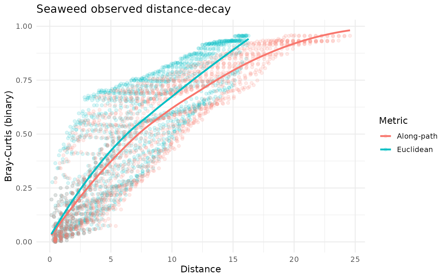
Interpolate unsampled seaweed sections
sea_interp <- simulate_between_observed(
  res_sea_obs,
  n_new_sites = 18,
  direction_bias = 0.35
)

ggplot() +
  geom_point(data = res_sea_obs$site_coords, aes(x, y), color = "black", size = 1.8) +
  geom_point(data = sea_interp$site_coords, aes(x, y), color = "red", size = 1.5, alpha = 0.8) +
  labs(title = "Seaweed observed sections (black) + interpolated unsampled sections (red)") +
  theme_minimal(base_size = 12)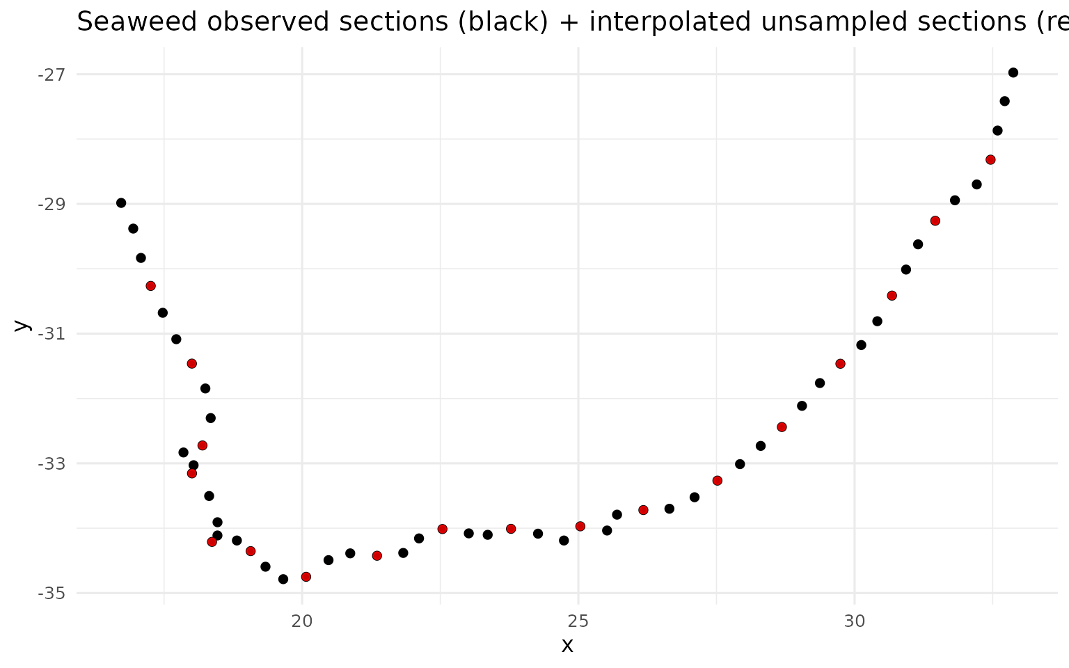
4) Advanced panels: observed vs interpolated
Doubs advanced panels
res_doubs_interp <- spesim_from_observed(
  abund_matrix = doubs_interp$abund_matrix,
  site_coords = doubs_interp$site_coords,
  site_env = doubs_interp$site_env,
  edges = build_network_edges(doubs_interp$site_coords, order_by = "linear_pos", directed = TRUE),
  directed = TRUE
)

res_doubs_obs_panel <- panel_ready_res(res_doubs_obs, max_species = 26L)
res_doubs_interp_panel <- panel_ready_res(res_doubs_interp, max_species = 26L)

generate_advanced_panel(res_doubs_obs_panel) +
  patchwork::plot_annotation(title = "Doubs observed data: advanced panel")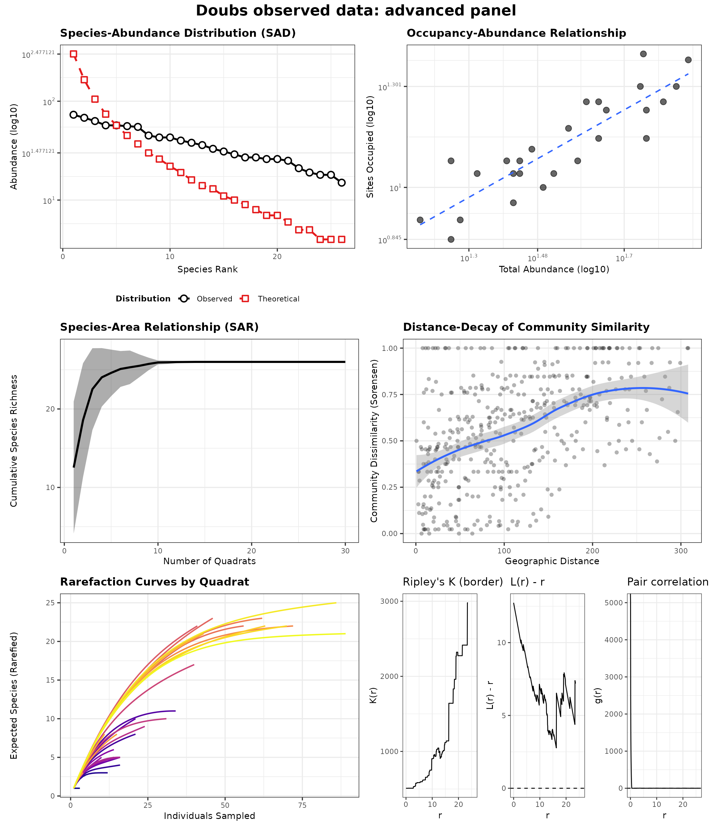
generate_advanced_panel(res_doubs_interp_panel) +
  patchwork::plot_annotation(title = "Doubs interpolated unsampled sites: advanced panel")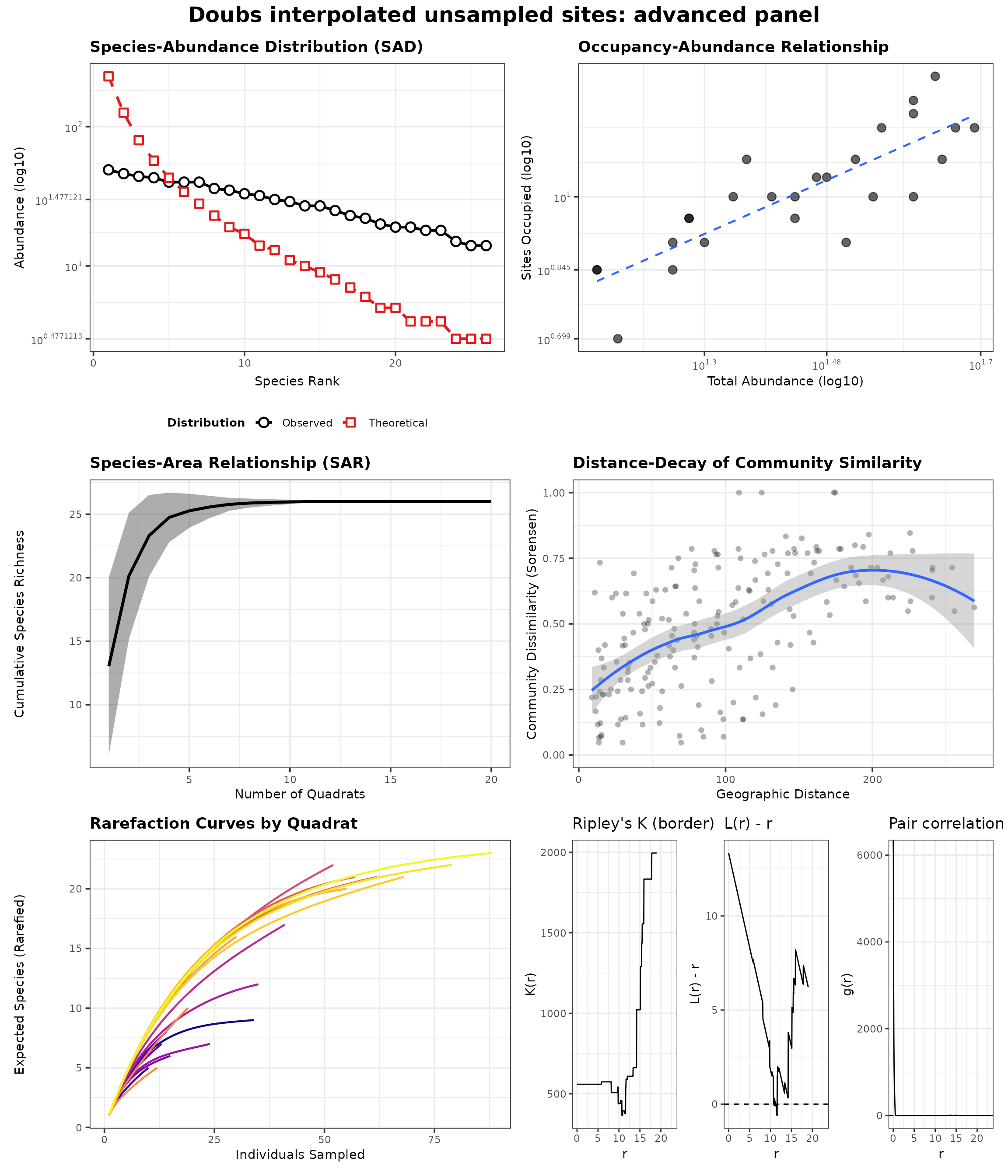
Seaweed advanced panels
res_sea_interp <- spesim_from_observed(
  abund_matrix = sea_interp$abund_matrix,
  site_coords = sea_interp$site_coords,
  site_env = sea_interp$site_env,
  edges = build_network_edges(sea_interp$site_coords, order_by = "linear_pos", directed = TRUE),
  directed = TRUE
)

res_sea_obs_panel <- panel_ready_res(res_sea_obs, max_species = 26L)
res_sea_interp_panel <- panel_ready_res(res_sea_interp, max_species = 26L)

generate_advanced_panel(res_sea_obs_panel) +
  patchwork::plot_annotation(title = "Seaweed observed data: advanced panel")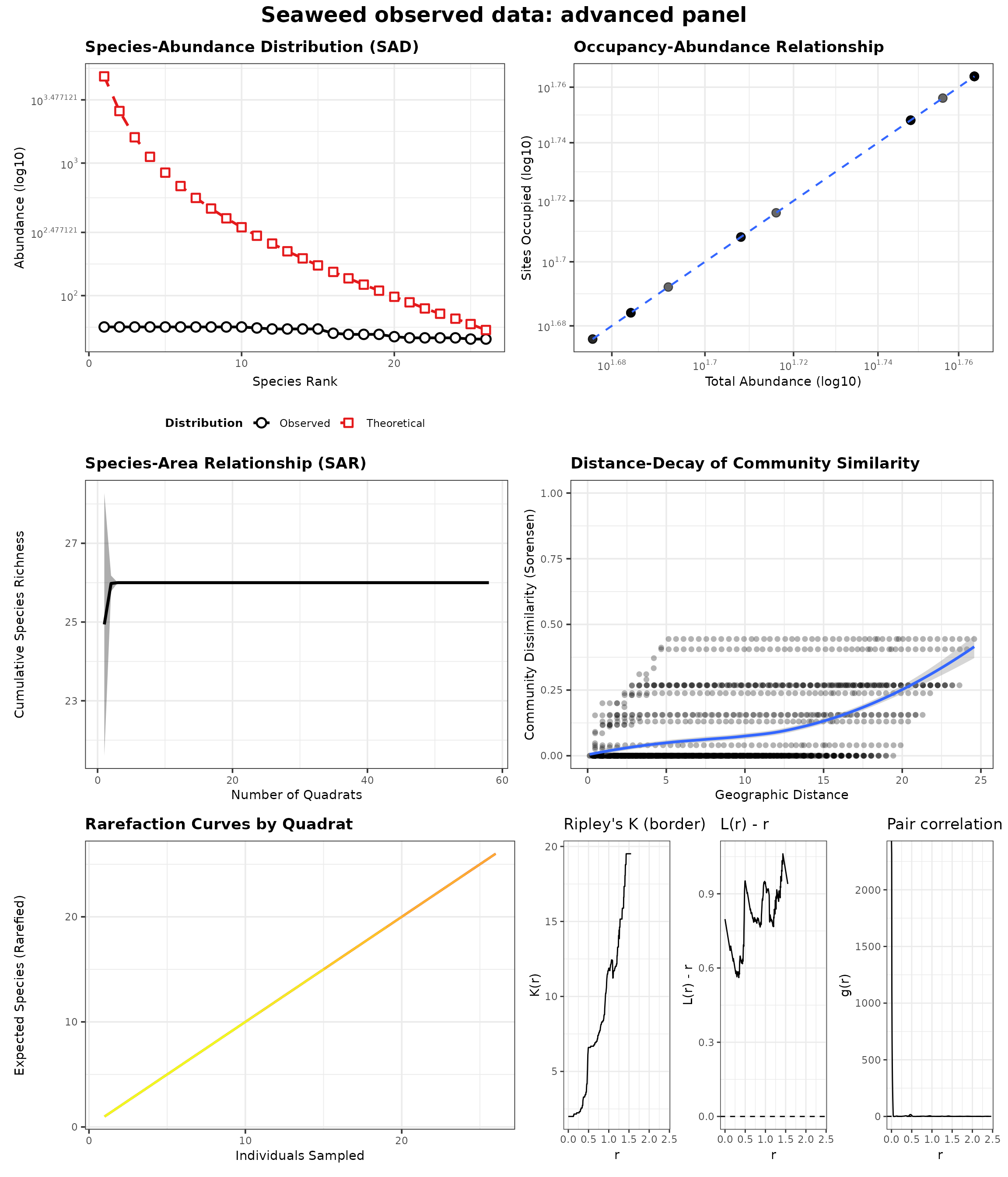
generate_advanced_panel(res_sea_interp_panel) +
  patchwork::plot_annotation(title = "Seaweed interpolated unsampled sections: advanced panel")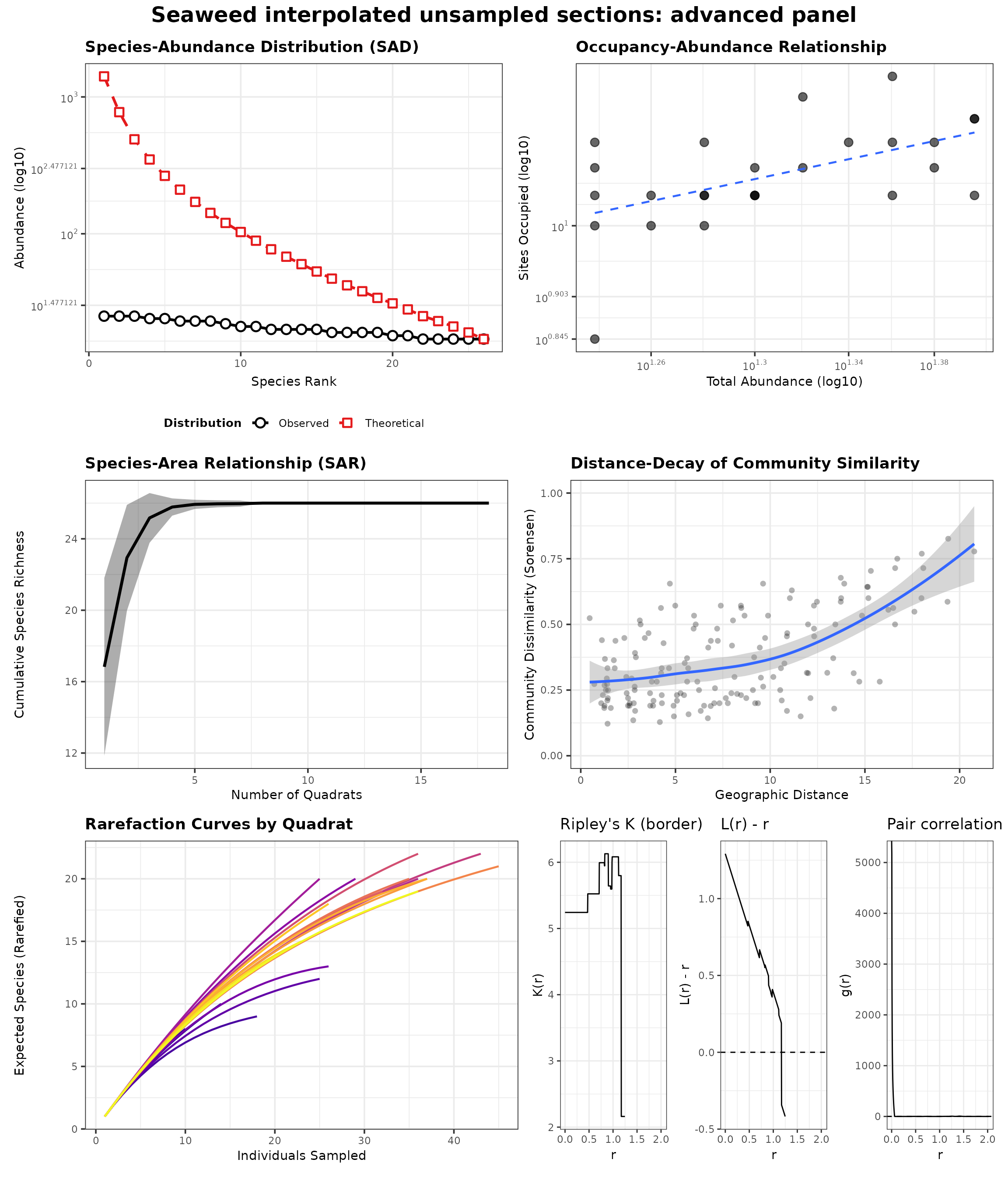
Practical notes
- The CSV paths are wired with
pkg_file(...), which resolvessystem.file("extdata/...", package = "spesim")for installed-package use and falls back toinst/extdata/...for source-tree rendering. - For Doubs and seaweed, observed species/environment tables are used
directly via
spesim_from_observed()(no new observed data are simulated). - Network connectivity is represented with explicit edges and used in along-path distance-decay calculations.
-
simulate_between_observed()provides first-pass interpolation into unsampled spaces between sampled units, with optional directional bias.