Chapter 10 Mapping with OpenStreetMap
“The only thing Google has failed to do, so far, is fail.”
— John Battelle
“I’m afraid that if you look at a thing long enough, it loses all of its meaning.”
— Andy Warhol
Now that we’ve seen how to produce complex maps with ggplot2 we are going to learn how to bring some freely-available maps—OpenStreetMaps—into the mix. Some kind hearted person has made a package for R that allows us to do this relatively easily. But that means we will need to install another new package.
After we learn how to use OpenStreetMap we will take some time to learn additional mapping techniques that we may want for creating publication quality figures.
10.1 OpenStreetMap
The package we will need for this tut is OpenStreetMap. It is a bit beefy so let’s get started on installing it now. Once it’s done we will activated the packages we need and load some site points for mapping.
# Load libraries
library(tidyverse)
Take a moment to look at the data we loaded. What does it show?
10.2 Mapping Cape Point
We will be creating our OpenStreetMap map in two steps. The first step is to use the openmap() function to define the area we want a map of, as well as what sort of map we want. In Google Maps and Google Earth we can switch from satellite view to map view, and we may do that in R and OpenStreetMap as well. For now we are only going to use the satellite view so that we may insert out own labels. But if we look in the help file we may see a description of all the different map types available. There are a bunch!
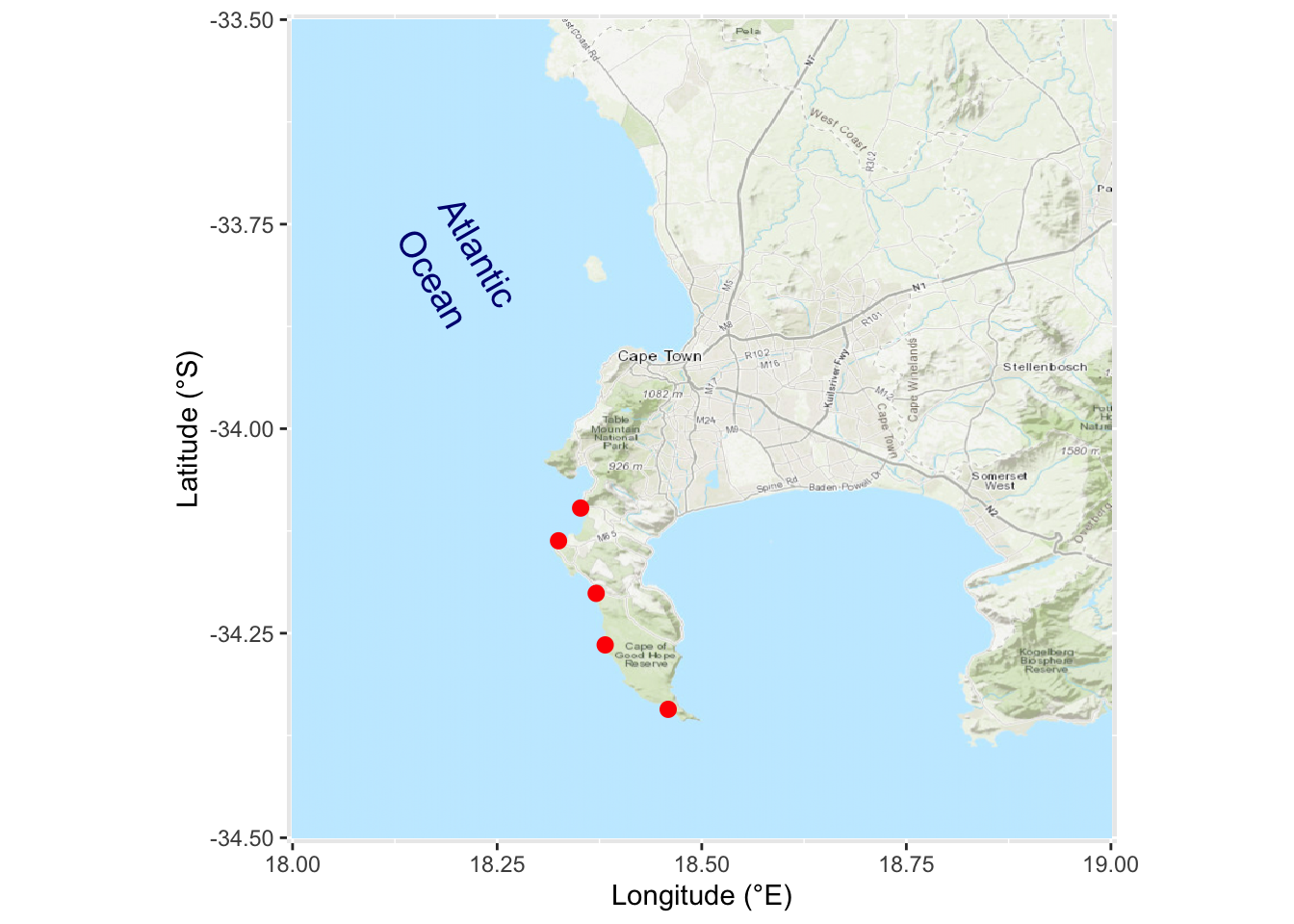
The openmap() function relies on a healthy internet connection to run. The downloading of OpenStreetMap maps can be a tenuous process without a stable connection. In the same sequence of steps we also add some points to indicate the spatial location of the kelp sampling sites (for the Laminaria and Ecklonia data), and the same annotations for the Atlantic Ocean that we first saw in Chapter 9. Here is how:
# load the location of the study sites
load("data/cape_point_sites.RData")

# define the spatial extent to OpenStreetMap
lat1 <- -34.5; lat2 <- -33.5; lon1 <- 18; lon2 <- 19

library(OpenStreetMap)

# other 'type' options are "osm", "maptoolkit-topo", "bing", "stamen-toner",
# "stamen-watercolor", "esri", "esri-topo", "nps", "apple-iphoto", "skobbler";
# play around with 'zoom' to see what happens; 10 seems just right to me
sa_map <- openmap(c(lat2, lon1), c(lat1, lon2), zoom = 10,
                  type = "esri-topo", mergeTiles = TRUE)

# reproject onto WGS84
sa_map2 <- openproj(sa_map)

# use instead of 'ggplot()'
sa_map2_plt <- OpenStreetMap::autoplot.OpenStreetMap(sa_map2) +
  annotate("text", label = "Atlantic\nOcean",
           x = 18.2, y = -33.8, size = 5.0, angle = -60, colour = "navy") +
  geom_point(data = cape_point_sites,
             aes(x = lon + 0.002, y = lat - 0.007), # slightly shift the points
             colour = "red", size =  2.5) +
  xlab("Longitude (°E)") + ylab("Latitude (°S)")
sa_map2_plt
Figure 10.1: Google map of Cape Point
The process seen in the code above is to treat the OpenStreetMap data we downloaded as though it is just any ordinary ggplot2 object. The same as the ones we created yesterday and today. For this reason we may use + to add new lines of conventional ggplot2 code to the map drawn by OpenStreetMap::autoplot.OpenStreetMap() in order to show site annotations, locations, etc.
Pretty cool huh?! You may do this for anywhere in the world just as easy as this. The only thing you need to keep in mind is that the lon/lat coordinates for OpenStreetMap appear to be slightly different than the global standard. This is why the x and y aes() values in the code above have a little bit added or subtracted from them. That one small issue aside, this is a nice quick workflow for adding your site locations to a neat map background. Play around with the different map types you can download and try it for any place you can think of.
10.3 Site labels
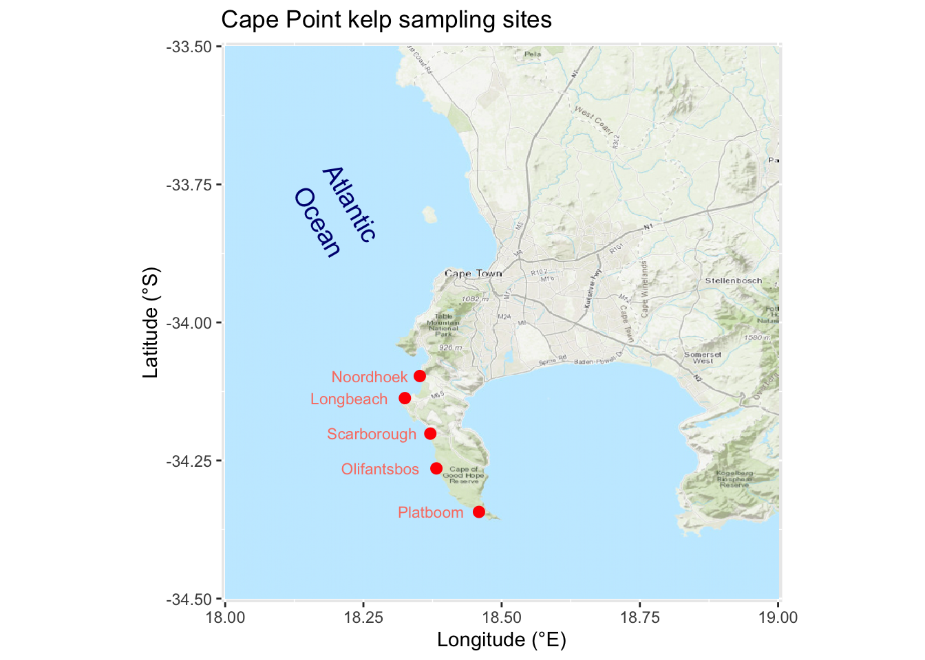
The previous figure shows our sites along Cape Point, which is great, but which site is which?! We need site labels. This is a relatively straightforward process, so we’ve given a complicated example of how to do so here. We already loaded the data in the file data/cape_point_sites.RData.
sa_map3_plt <- sa_map2_plt +
  geom_text(data = cape_point_sites, # Choose dataframe
            aes(lon+0.002, lat-0.007, label = site), # Set aesthetics
            hjust = 1.15, vjust = 0.5, # Adjust vertical and horizontal
            size = 3, colour = "salmon") + # Adjust appearance
  ggtitle("Cape Point kelp sampling sites")
sa_map3_plt
Figure 10.2: Google map of Cape Point with site points labeled
10.4 DIY maps
Now that we have learned how to make conventional maps, as well as fancy OpenStreetMap maps, it is time for us to branch out once again at let our creative juices flow. Please group up as you see fit and create your own beautiful map of wherever you like. Bonus points for faceting in additional figures showing supplementary information. Feel free to use either conventional maps or the OpenStreetMaps alternative. Same as yesterday, we will be walking the room to help with any issues that may arise.
10.5 Session info
installed.packages()[names(sessionInfo()$otherPkgs), "Version"]R> OpenStreetMap forcats stringr dplyr purrr
R> "0.3.4" "0.5.1" "1.4.0" "1.0.7" "0.3.4"
R> readr tidyr tibble ggplot2 tidyverse
R> "1.4.0" "1.1.3" "3.1.2" "3.3.4" "1.3.1"