Chapter 9 Confidence intervals
A confidence interval (CI) tells us within what range we may be certain to find the true mean from which any sample has been taken. If we were to repeatedly sample the same population over and over and calculated a mean every time, the 95% CI indicates the range that 95% of those means would fall into.
9.1 Calculating confidence
Input <- ("
Student  Sex     Teacher  Steps  Rating
a        female  Jacob    8000   7
b        female  Jacob    9000  10
c        female  Jacob   10000   9
d        female  Jacob    7000   5
e        female  Jacob    6000   4
f        female  Jacob    8000   8
g        male    Jacob    7000   6
h        male    Jacob    5000   5
i        male    Jacob    9000  10
j        male    Jacob    7000   8
k        female  Sadam    8000   7
l        female  Sadam    9000   8
m        female  Sadam    9000   8
n        female  Sadam    8000   9
o        male    Sadam    6000   5
p        male    Sadam    8000   9
q        male    Sadam    7000   6
r        female  Donald   10000  10
s        female  Donald    9000  10
t        female  Donald    8000   8
u        female  Donald    8000   7
v        female  Donald    6000   7
w        male    Donald    6000   8
x        male    Donald    8000  10
y        male    Donald    7000   7
z        male    Donald    7000   7
")

data <- read.table(textConnection(Input),header = TRUE)
summary(data)
R> Student Sex Teacher Steps
R> Length:26 Length:26 Length:26 Min. : 5000
R> Class :character Class :character Class :character 1st Qu.: 7000
R> Mode :character Mode :character Mode :character Median : 8000
R> Mean : 7692
R> 3rd Qu.: 8750
R> Max. :10000
R> Rating
R> Min. : 4.000
R> 1st Qu.: 7.000
R> Median : 8.000
R> Mean : 7.615
R> 3rd Qu.: 9.000
R> Max. :10.000library(rcompanion)
# ungrouped data is indicated with a 1 on the right side of the formula, or the group = NULL argument.
groupwiseMean(Steps ~ 1,data = data, conf = 0.95, digits = 3)R> .id n Mean Conf.level Trad.lower Trad.upper
R> 1 <NA> 26 7690 0.95 7170 8210# one-way data
groupwiseMean(Steps ~ Sex, data = data, conf = 0.95,digits = 3)R> Sex n Mean Conf.level Trad.lower Trad.upper
R> 1 female 15 8200 0.95 7530 8870
R> 2 male 11 7000 0.95 6260 7740# two-way data
groupwiseMean(Steps ~ Teacher + Sex, data = data, conf = 0.95,digits = 3)R> Teacher Sex n Mean Conf.level Trad.lower Trad.upper
R> 1 Donald female 5 8200 0.95 6360 10000
R> 2 Donald male 4 7000 0.95 5700 8300
R> 3 Jacob female 6 8000 0.95 6520 9480
R> 4 Jacob male 4 7000 0.95 4400 9600
R> 5 Sadam female 4 8500 0.95 7580 9420
R> 6 Sadam male 3 7000 0.95 4520 9480# by bootstrapping
groupwiseMean(Steps ~ Sex,
data = data,
conf = 0.95,
digits = 3,
R = 10000,
boot = TRUE,
traditional = FALSE,
normal = FALSE,
basic = FALSE,
percentile = FALSE,
bca = TRUE)R> Sex n Mean Boot.mean Conf.level Bca.lower Bca.upper
R> 1 female 15 8200 8200 0.95 7530 8670
R> 2 male 11 7000 6990 0.95 6270 7550groupwiseMean(Steps ~ Teacher + Sex,
data = data,
conf = 0.95,
digits = 3,
R = 10000,
boot = TRUE,
traditional = FALSE,
normal = FALSE,
basic = FALSE,
percentile = FALSE,
bca = TRUE)R> Teacher Sex n Mean Boot.mean Conf.level Bca.lower Bca.upper
R> 1 Donald female 5 8200 8200 0.95 6800 9000
R> 2 Donald male 4 7000 7000 0.95 6000 7500
R> 3 Jacob female 6 8000 8000 0.95 6830 8830
R> 4 Jacob male 4 7000 7000 0.95 5000 8000
R> 5 Sadam female 4 8500 8510 0.95 8000 8750
R> 6 Sadam male 3 7000 7000 0.95 6000 7670These upper and lower limits may then be used easily within a figure.
# Load libraries
library(tidyverse)

# Create dummy data
r_dat <- data.frame(value = rnorm(n = 20, mean = 10, sd = 2),
                    sample = rep("A", 20))

# Create basic plot
ggplot(data = r_dat, aes(x = sample, y = value)) +
  geom_errorbar(aes(ymin = mean(value) - sd(value), ymax = mean(value) + sd(value))) +
  geom_jitter(colour = "firebrick1")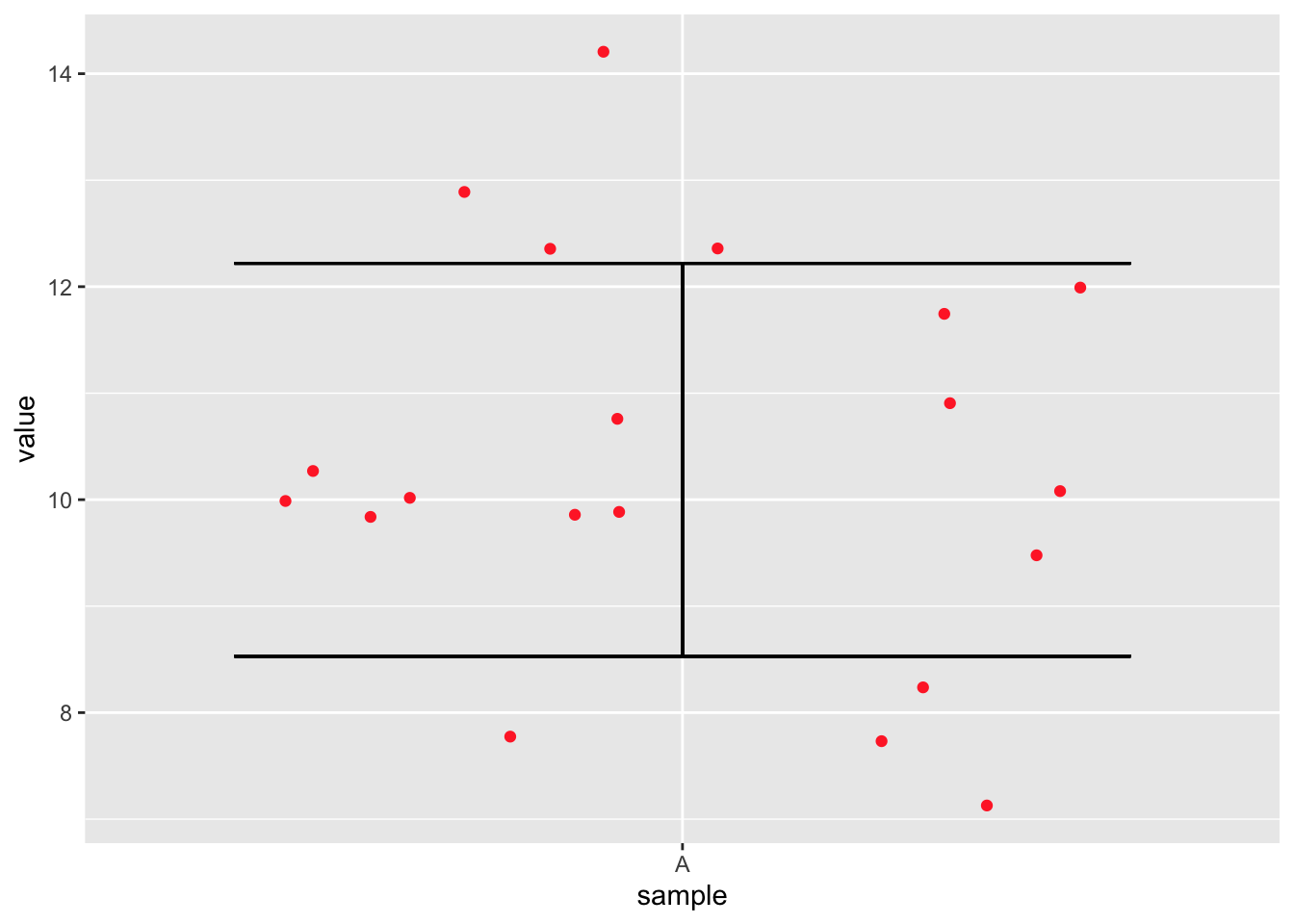
Figure 9.1: A very basic figure showing confidence intervals (CI) for a random normal distribution.
Task: How would we apply this to more than one sample set? Do so now.
9.2 CI of compared means
AS stated above, we may also use CI to investigate the difference in means between two or more sample sets of data. We have already seen this in Chapter 7, ANOVA, but we shall look at it again here with our now expanded understanding of the concept.
# First calculate ANOVA of seapl length of different iris species
iris_aov <- aov(Sepal.Length ~ Species, data = iris)

# Then run a Tukey test
iris_Tukey <- TukeyHSD(iris_aov)

# Lastly use base R to quickly plot the results
plot(iris_Tukey)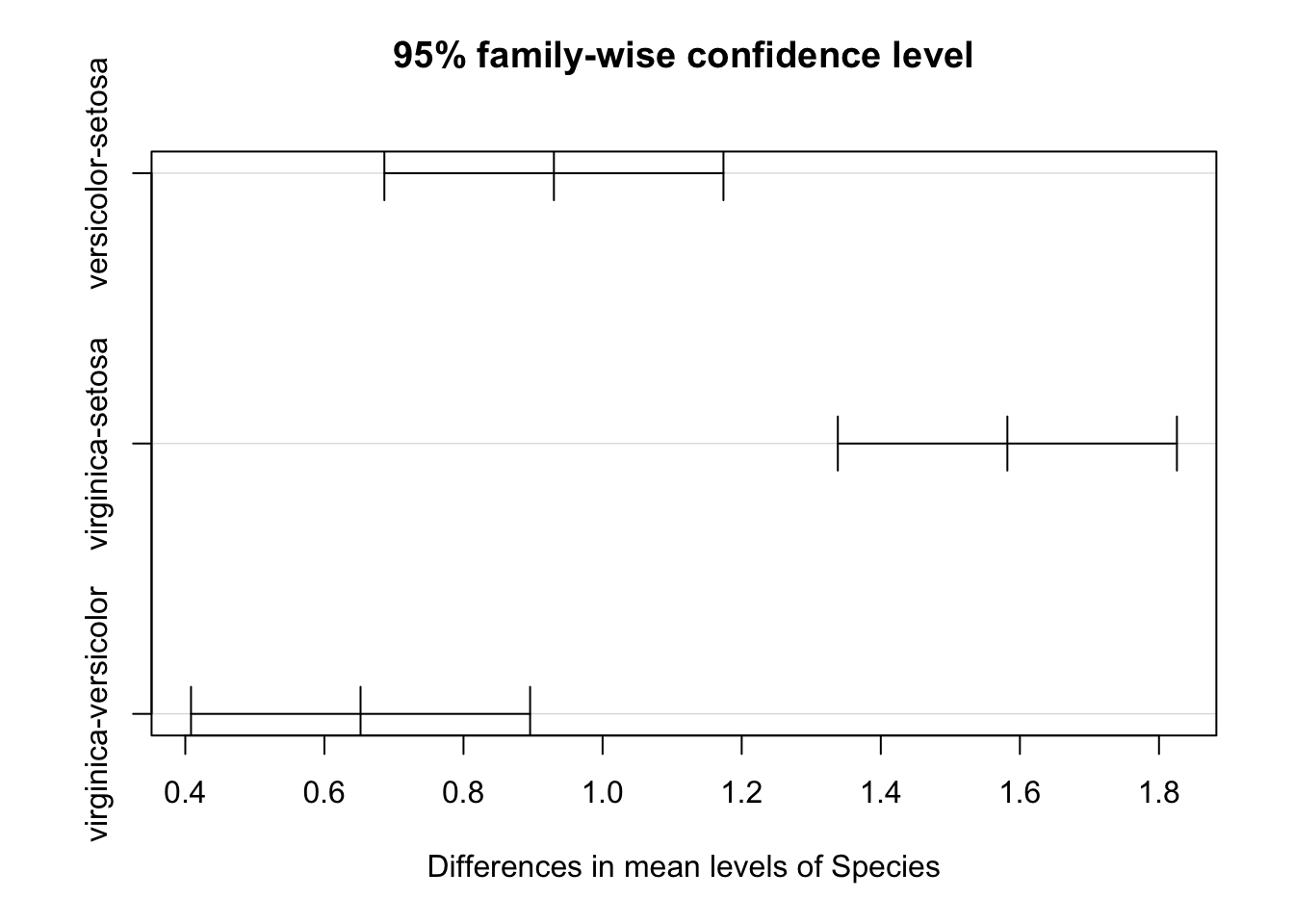
Figure 9.2: Results of a post-hoc Tukey test showing the confidence interval for the effect size between each group.
Task: Judging from the figure above, which species have significantly different sepal lengths?
9.3 Harrell plots
The most complete use of CI that we have seen to date is the Harrell plot. This type of figure shows the distributions of each sample set in the data as boxplots in a lower panel. In the panel above those boxplots it then lays out the results of a post-hoc Tukey test. This very cleanly shows both the raw data as well as high level statistical results of the comparisons of those data. Thanks to the magic of the Internet we may create these figures with a single line of code. This does however require that we load several new libraries.
# The easy creation of these figures has quite a few dependencies
library(tidyverse)
library(lsmeans)
library(Hmisc)
library(broom)
library(car)
library(data.table)
library(cowplot)
source("data/fit_model.R")
source("data/make_formula_str.R")
source("data/HarrellPlot.R")

# Load data
ecklonia <- read_csv("data/ecklonia.csv")

# Create Harrell Plot
HarrellPlot(x = "site", y = "stipe_length", data = ecklonia, short = T)[1]
R> $gg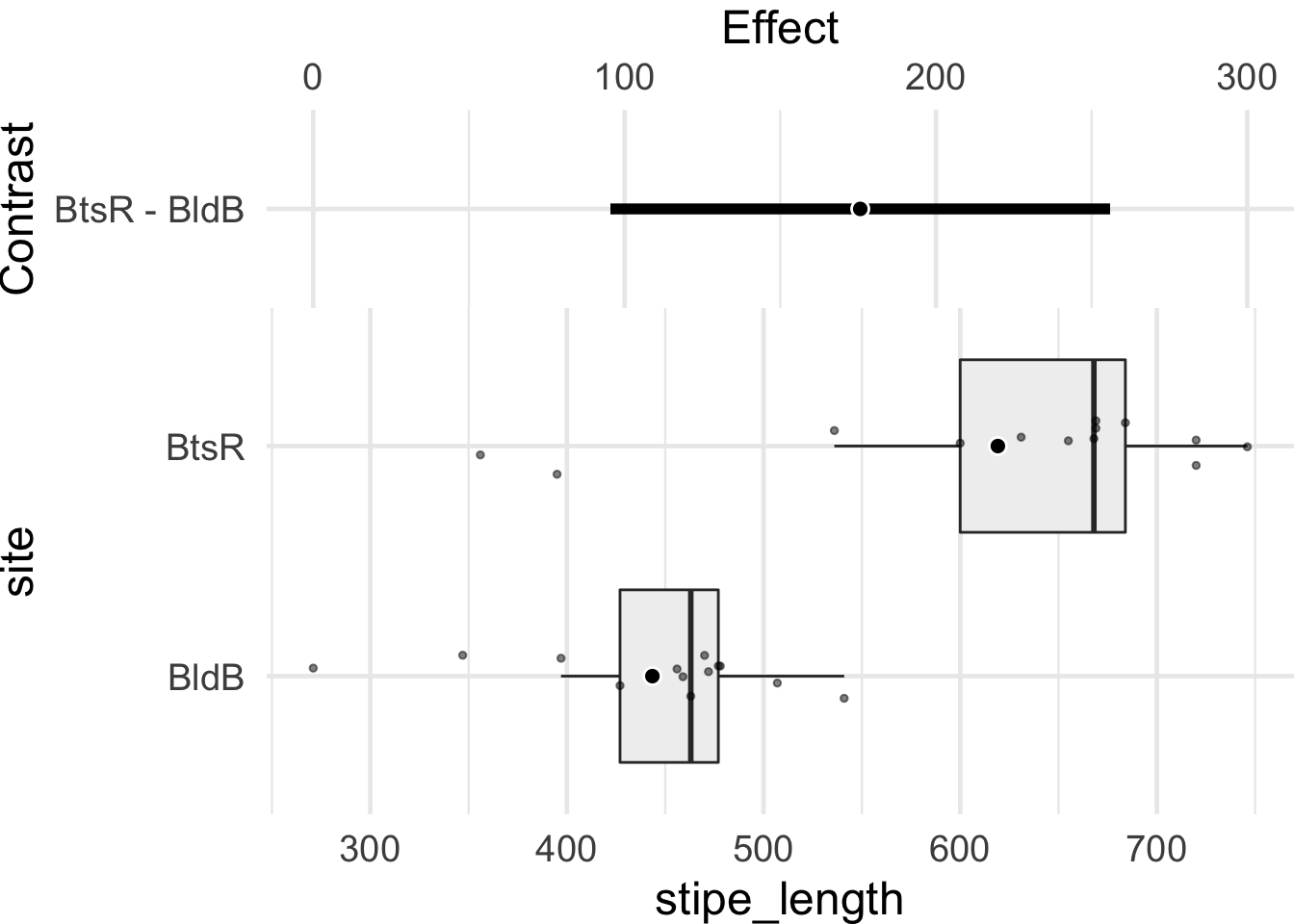
Figure 9.3: Harrell plot showing the distributions of stipe lengths (cm) of the kelp Ecklonia maxima at two different sites in the bottom panel. The top panel shows the confidence interval of the effect of the difference between these two sample sets based on a post-hoc Tukey test.
Task: There are a lot of settings for
HarrePlot(), what do some of them do?
The above figure shows that the CI of the difference between stipe lengths (cm) at the two sites does not cross 0. This means that there is a significant difference between these two sample sets. But let’s run a statistical test anyway to check the results.
# assumptions
ecklonia %>%
  group_by(site) %>%
  summarise(stipe_length_var = var(stipe_length),
            stipe_length_Norm = as.numeric(shapiro.test(stipe_length)[2]))
R> # A tibble: 2 x 3
R> site stipe_length_var stipe_length_Norm
R> <chr> <dbl> <dbl>
R> 1 Batsata Rock 14683. 0.0128
R> 2 Boulders Beach 4970. 0.0589# We fail both assumptions...
# non-parametric test
wilcox.test(stipe_length ~ site, data = ecklonia)R>
R> Wilcoxon rank sum test with continuity correction
R>
R> data: stipe_length by site
R> W = 146, p-value = 0.001752
R> alternative hypothesis: true location shift is not equal to 0The results of our Wilcox rank sum test, unsurprisingly, support the output of HarrelPlot().
9.4 Exercises
9.4.1 Exercise 1
Load a new dataset and create a Harrell plot from it based on values of your choosing. What does the Harrell plot show?